Besides Historical Returns
Beyond historical returns: a multidimensional framework for expected returns across asset classes, strategy styles, and risk factors. Based on Anti Ilmanen
The traditional paradigm treats historical returns as expected returns and focuses too narrowly on asset class allocation. This leads to decision-making that is blind to everything except past performance. A more complete approach requires multidimensional inputs: historical average returns, financial and behavioral theories, forward-looking market indicators, and discretionary views.
When expected returns are discussed, they are almost always framed through asset classes. But this oversimplifies financial markets. Strategy styles and risk factors are equally valid, and mutually exclusive, perspectives for forecasting returns. Viewing markets through an asset class lens alone (equities, bonds, credit, commodities, hedge funds, private equity) naturally raises questions about the classic 60/40 portfolio. That portfolio relies heavily on a single source of excess return (the equity risk premium), which results in highly concentrated risk: more than 90% of portfolio volatility is attributable to equities. 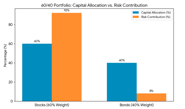 Variance decomposition of a 60/40 portfolio: equities dominate total portfolio risk This concentration is straightforward to derive from the weighted covariance of the portfolio. For a two-asset portfolio of stocks and bonds:
The contribution of stocks to total variance is:
\[w_s \frac{\partial \sigma_p^2}{\partial w_s} = 2 w_s^2 \sigma_s^2 + 2 w_s w_b \sigma_s \sigma_b\]By Euler’s theorem, since \(\sigma_p^2\) is homogeneous of degree 2:
\[w_s \frac{\partial \sigma_p^2}{\partial w_s} + w_b \frac{\partial \sigma_p^2}{\partial w_b} = 2\sigma_p^2\]The contributions are exhaustive and distinct, and the stock contribution dominates at 60/40 weights given typical volatility and correlation parameters.
Structure of Expected Return Inputs
Each of the four inputs below applies across all three perspectives: asset classes, strategy styles, and risk factors.
- Historical average returns
- Financial and behavioral theories
- Forward-looking market indicators
- Discretionary views
Historical Performance
Historical returns are a natural starting point for forecasting expected returns. The underlying assumption is that expected returns are constant over time, so the long-run historical average serves as a good estimate of the expected future return. The emphasis, however, is on starting point.
In the short run, news and idiosyncratic noise distort expected returns, but they tend to cancel out over longer horizons. That said, any sample period may in hindsight be biased and thus unrepresentative of true market expectations, particularly if the sample begins or ends at a period of exceptionally high or low valuations.
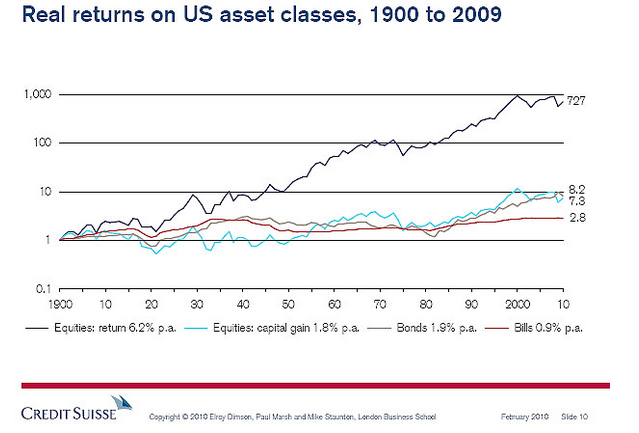 Real cumulative returns on US equities, bonds, and bills, 1900–2009. Source: Dimson, Marsh & Staunton / Credit Suisse (2010)
A commonly cited example: it is often said that equities outperform fixed income, and this holds across most countries over the past century. The compound average real return for global equities between 1990 and 2009 was 5.4%, which exceeded long-term government bonds and short-dated treasury bills by 3.7% and 4.4% respectively. But this stylised fact is complicated by lived experience: the belief that stocks beat bonds over any 20–30 year horizon is challenged by specific historical periods and starting valuations.
Strategy Styles
Beyond asset classes, different strategy styles have proven profitable across multiple markets: value (overweighting assets that appear cheap on valuation metrics, underweighting expensive ones), carry (overweighting high-yielding assets, underweighting low-yielding ones), and momentum (overweighting recent outperformers, underweighting recent laggards). It should be noted that selection bias and overfitting have overstated the profitability of many simulated results.
Backtests: Value, Carry, and Momentum
Value
The hypothesis was that a simple low P/E strategy does not exploit mispricings but instead harvests risk premia: returns that are not competed away because they require investors to bear real, clusterable risks. To test this, the strategy ranked S&P 500 stocks by P/E, invested in the lowest-valued names within a five-to-thirty band, applied a 200-day SMA filter on SPY to avoid bear markets (with a two-day confirmation below the average), and exited on a 12% stop loss or two consecutive days below the moving average. The backtest ran from October 2018 to May 2026, beginning near a post-2009 peak when SPY itself traded at a P/E of 21–22.
Results: alpha –0.004, beta 0.362, Sharpe 0.161, probabilistic Sharpe (PSR at 1%) 0.161. Maximum drawdown was –34%, while SPY returned approximately 130–140% over the same period. The negative alpha indicates that after accounting for market risk, the strategy produced less return than expected; it did not identify mispriced stocks but instead selected names that bore correctly priced risks.
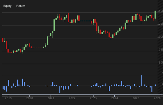 Value strategy (low P/E, 200-day SMA filter) vs SPY, October 2018 – May 2026
The beta dynamics are instructive. In normal periods beta was low, but during value rotations it spiked. In Q4 2018, the strategy lost 26% and its beta turned –2, meaning it amplified bear market losses. When the Fed pivoted in early 2019, Powell halted hikes in January and began signalling cuts. The market recovered sharply, pulling value stocks with it, but the strategy’s upside was capped by the prior drawdown.
A simple P/E screen is blind to structural impairment (free cash flow trends, competitive position, revenue trajectory) and to macroeconomic conditions. In April 2022, the strategy entered Rio Tinto just as the Fed began hiking aggressively. The Russia–Ukraine war had inflated commodity prices, making RIO appear cheap, but iron ore subsequently collapsed. Regional banks (TFC, CFG, KEY, HBAN) were similarly selected for their low P/Es, yet these holdings multiplied beta significantly; in March 2023, each collapsed simultaneously during the SVB crisis, generating losses of approximately $12,000.
Specific examples illustrate why the strategy fails to find mispricings. The market did not misprice Macy’s: it was pricing in secular decline from e-commerce, liability-laden mall locations, and an unsustainable debt load. The low P/E was the market’s correct risk premium for holding a structurally impaired business. CenturyLink offered a high yield and low P/E, but the market was pricing in dividend sustainability risk: an 8% yield is the market’s compensation for the probability of a cut, which arrived in February 2019 at –54%, collapsing the share price and generating a loss of $2,415. For energy and materials names (RIO, VLO, FANG, PXD), combined losses were approximately $12,000. Commodity companies always appear cheap at the peak of their earnings cycle: trailing P/E is depressed because earnings are inflated by high commodity prices. When iron ore fell, crack spreads compressed, and natural gas collapsed, those earnings evaporated. The market was pricing risk correctly; the strategy was accepting it without adequate compensation.
Four follow-up questions worth pursuing:
Am I being adequately compensated for the risks I am accepting? A Sharpe of 0.161 answers: barely. The value risk premium in this implementation is too thin relative to the volatility and drawdown it demands. Either the premium needs improvement (better quality filters, sector caps) or the risk needs reduction (smaller positions in fragile sectors, a momentum overlay to avoid value traps).
Are the risks I am accepting correlated with each other? In March 2023, every regional bank in the portfolio collapsed simultaneously. In Q4 2018, every retail and telecom position fell together. Risk premia that appear diversified by company name can be concentrated in a single underlying risk factor. Holding ten regional banks is not diversification; it is ten expressions of the same systemic banking risk.
In what macro regime does this risk premium get paid, and in what regime does it get collected back? The data answer this precisely. The value risk premium is paid in reflation regimes (rates rising from low levels, economic recovery, tightening credit spreads). It is collected back in credit stress regimes (banking crises, rate shocks, recession fears).
What is the right price to pay for this risk premium? Historical averages are a starting point, not a destination. The value premium itself varies over time. After a decade of growth outperforming value (2010–2020), the value premium was compressed. Entering in October 2018, at the tail end of that compression, meant starting when the premium was at its thinnest. The value outperformance of 2021–2022 was a partial normalisation of that premium, not alpha.
Carry
The logic is pure carry: go long the highest-dividend-yielding stocks in the S&P 500 and rebalance monthly, collecting income while assuming prices remain stable. The backtest runs from October 2018 to May 2026.
Results: CAGR 8.34%, total return 78.85%, maximum drawdown –43.6%, Sharpe 0.241, PSR (1%) 2.74%, alpha –0.010, beta 0.636. The strategy generates more absolute return than value or momentum but still underperforms the benchmark on a risk-adjusted basis.
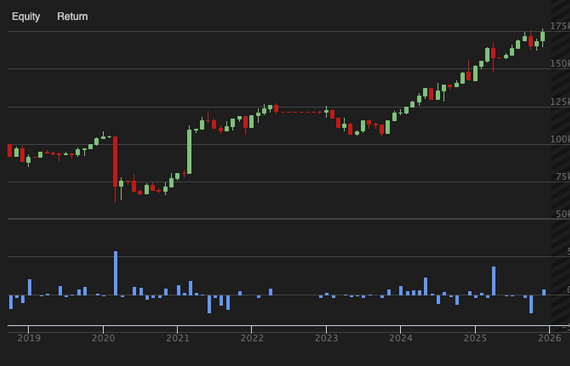 Carry strategy (highest-yielding S&P 500 stocks, monthly rebalance) vs SPY, October 2018 – May 2026
The sector story distinguishes two kinds of high yield. Winners are infrastructure carry: pipelines (WMB, OKE, KMI), tobacco (MO, PM), utilities (SO), with contractual or inelastic revenue streams. Losers are cyclical carry: healthcare REITs, gaming, mortgage REITs, and E&P energy, where dividends disappear when the underlying business conditions break. A naive yield screen cannot distinguish the two.
Alpha of –0.010 makes the conclusion clear. The 8.34% CAGR is not alpha; it is the equity risk premium collected through a high-beta, income-focused vehicle. Three identifiable risk premia are being accepted: the dividend risk premium (high-dividend payers are discounted by investors who fear cuts), the income volatility premium (yield-focused investors exit simultaneously in downturns), and the sector concentration premium (pipelines, tobacco, and utilities trade at permanent valuation discounts). None of these represent mispricings; they are the correct price for identifiable, persistent risks.
Momentum
The logic is pure trend following: go long the best-performing stocks in the S&P 500 over the prior month, rebalance monthly, exit on a –12% stop loss or if SPY falls below its 200-day SMA. The backtest runs from October 2018 to May 2026.
Academic momentum research traditionally uses a 12-month lookback with annual rebalancing, capturing the prior year’s winners for the following year. That slower frequency filters out short-lived spikes. Monthly rebalancing is deliberately more aggressive: resetting every month forces the strategy to continuously buy whatever has risen most recently, including meme stocks, event-driven spikes, and fragile trends. This is not a design flaw but a feature that reveals the strategy’s nature as a risk-premium harvester. At monthly frequency, the strategy is not identifying durable winners; it is accepting the risk of holding whatever is most prone to sudden reversal, and earning (or not) the premium for doing so.
Results: CAGR 5.51%, total return 47.64%, maximum drawdown –47.5%, Sharpe 0.134, PSR (1%) 1.14%, beta 0.279, the lowest of the three strategies.
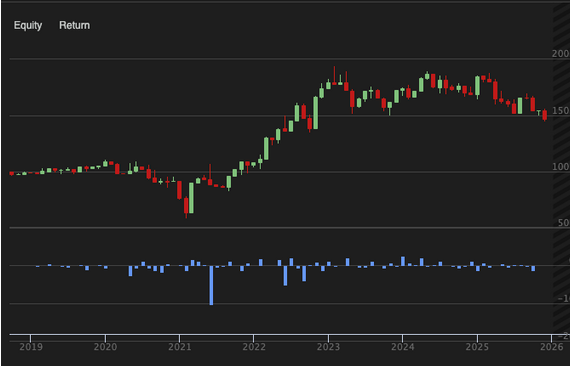 Momentum strategy (prior-month top performers, monthly rebalance) vs SPY, October 2018 – May 2026
The specific risk being harvested is trend continuation risk: the risk that a price trend reverses abruptly before the position can be exited. Academic literature identifies two components: the underreaction premium (investors are slow to incorporate new information, so trends persist) and the crash premium (trends occasionally reverse violently when crowded positions unwind). Monthly rebalancing exposes the strategy fully to both. Small, steady gains accumulate when underreaction persists (as in 2022), while large sudden losses arrive when crowded momentum positions crash (as with GME or Kodak). The 5.51% CAGR is what remains after both sides of that trade have settled.
2022 demonstrates momentum working as intended. While the S&P 500 fell 18%, the strategy gained $73,121, its best single year across all three strategies. The Russia–Ukraine war created a sustained macro trend in energy, defense, and select commodities; the monthly filter captured and held it through the run.
A shared conclusion across all three strategies: these results do not imply that the strategies have been competed away. If returns reflect risk premia rather than market inefficiencies, they will continue to deliver positive future excess returns, though not necessarily profitability after costs, leverage, and implementation frictions.
A Note on Volatility and Expected Returns
The relationship between volatility and expected returns is non-trivial. In the most basic sense, a strategy that sells equity index options earns a positive long-run excess return, justified by the nature of its risk-bearing (selling financial catastrophe insurance). However, the most volatile assets within each asset class (growth stocks, 40-year treasuries, CCC-rated corporate bonds) tend to offer the lowest long-run risk-adjusted returns.
This pattern traces back to two well-documented biases: investors’ lottery-seeking tendency, which leads to overpaying for assets with jackpot-like upside, and leverage constraints, which prevent many investors from boosting returns by levering stable assets and instead drive them toward inherently volatile ones. The practical implication is that one is often better served by avoiding inherently volatile assets and instead levering up stable ones, rather than overpaying for assets whose high valuations reflect extrapolated past growth rates.
Financial and Behavioral Theories
Until the 1950s, financial theory was largely undeveloped. Over the following three decades, it evolved through a series of relatively simple models built on highly restrictive assumptions: the single-factor CAPM, the efficient market hypothesis, and constant risk premia. These frameworks were designed to explain asset prices and expected returns in a tractable way.
Early asset pricing theory held that investors set prices such that an asset’s cost equals its expected benefit: the market price of any asset equals the expected sum of future cash flows discounted to present value. The critical question became what should determine the discount rate. Assuming rational, risk-averse investors, the discount rate cannot simply be the riskless rate unless the cash flow itself is riskless. Instead, it must reflect the required return for the riskiness of the asset’s expected future cash flows, capturing both the nature of the risk and investors’ aversion to it.
CAPM formalised this: an asset’s risk is fully captured by its market beta, and investor risk aversion determines the size of the market risk premium. Each asset’s expected excess return equals its beta multiplied by the common market risk premium. Differences in expected returns across assets reflect only differences in betas, and one can increase expected return by bearing more market risk.
The Security Market Line (SML) captures this relationship precisely:
\[E[R_i] = R_f + \beta_i \bigl(E[R_M] - R_f\bigr)\]The risk-free rate \(R_f\) provides the base compensation for the time value of money. The market risk premium \((E[R_M] - R_f)\) represents the average additional return demanded for bearing average market risk. Beta \(\beta_i\) scales this premium to reflect the asset’s specific sensitivity to market movements: assets with \(\beta_i > 1\) are expected to be more volatile than the market and receive a proportionally larger premium; assets with \(\beta_i < 1\) receive less. The structure of the equation formalises a core theoretical claim: only systematic (market) risk is rewarded, while idiosyncratic risk is assumed to be diversified away and therefore uncompensated.
But these theories do not reflect real markets. High-beta stocks, much like high-volatility assets, offer no return advantage, and perhaps the reverse. The assumption of constant risk premia became particularly difficult to sustain after the boom-bust cycles of the late 20th and early 21st centuries.
If investors want to earn returns above the riskless rate, the most reliable path is to bear risks the market rewards with a premium. The simple story of a single risk factor, constant expected returns, and rational players is outdated. Returns have multiple drivers, and while market beta still explains a large share of risk, exposure to inflation, illiquidity, and tail risks all influence how assets are rewarded. The interrelations between factors also matter: portfolio diversification is more effective when return sources are independent or, better still, negatively correlated.
Expected return differentials depend less on standalone volatility than is commonly assumed. Many investors view the risk-reward tradeoff as determined by an asset’s volatility in isolation: stocks are more volatile than bonds, therefore they deserve higher long-run returns. This points in the right direction: risk does influence expected returns, but it oversimplifies. Each asset reflects a bundle of risk factors plus idiosyncratic risk that can be diversified away and therefore should not be rewarded. Only systematic risks command a premium, and the premium differs depending on which systematic factors are the source of the volatility.
A key theme from rational asset pricing is that assets and factors which perform poorly in bad times (crises, recessions) warrant high required returns. Safe havens that perform well in bad times, by contrast, command low risk premia. Certain assets deserve high expected returns (particularly in good times) precisely because they tend to deliver terrible returns when it hurts investors most.
Strategies with asymmetric risk profiles exhibit similar characteristics: selling tail insurance, writing options on equity indices, carry trading, and harvesting illiquidity premia all hold justifiably high long-run expected returns, but the losses are concentrated in rare, severe episodes. Trend following, by contrast, has a surprisingly different profile: it has shown a consistent record as a partial safe haven, delivering relatively well in periods of sustained market stress.
Forward-Looking Market Indicators
Forward-looking indicators are generally superior to historical averages for estimating expected returns because they are time-varying, a more realistic property. But they are not definitive. Even when two investors agree that long-term market returns reflect the sum of starting yield and growth prospects, their estimates can diverge sharply in practice.
The time-varying nature of expected returns makes historical averages misleading in specific episodes. Stock prices were unusually elevated in 2000: historical averages pointed to continued strong growth, but prospective returns were low. The halving of global equity prices between 2007 and 2008, conversely, created conditions for high long-term returns. Generalising: empirical evidence shows that near-term returns on risky assets tend to be relatively high near recessions and other troughs, and relatively low around peaks. This countercyclical pattern can be explained through both rational and behavioural lenses.
Rationally, ex-ante returns are time-varying risk premia: the amount of risk in the market, or investors’ aversion to it, or both, fluctuate over time. This logic generalises beyond equities; the inflation risk premium in nominal bonds was substantially higher in the 1980s than in the 2000s. When salient adverse events materialise for any given risk factor, the ex-ante premium tends to widen sharply and then gradually decay from elevated levels. The rate of that decay is itself an open empirical question.
Discretionary (View-Based) Expected Returns
There is little to add here that will be broadly useful. Alpha is a zero-sum game: mispricings and other sources of alpha tend to be competed away quickly, as profitable strategies attract capital, distorting returns asymmetrically until the edge effectively disappears. Active management follows the same trajectory. Superior managers surely exist, but identifying them in advance or becoming one is largely a function of accumulated experience and is not easily replicable from theory alone.
Notes
Diversification is a powerful tool, particularly when applied across complementary perspectives: strategy styles and risk factors rather than asset classes alone. Value and momentum strategies, for example, are negatively correlated; combining them produces much smoother return streams than either style in isolation. Negatively correlated return sources are among the most powerful diversifiers available and deserve deep study.
Diversifying directional market risk is considerably harder. Safe havens tend to be either expensive or unreliable over time.