CBOT Corn Futures Strategy: A Bottom Up Factor Framework

What should a corn futures contract be worth?

A simple answer would look only at the price chart and try to predict the next move from past returns. Or one could think of the process and realise corn futures are not just financial time series. They are contracts linked to a physical commodity that must be planted, grown, harvested, stored, consumed, exported, processed, fed to livestock, and sometimes delivered against a specific futures month.

So the better first question is not:

\[\text{Will corn go up or down tomorrow?}\]

The better first question is:

\[\text{What physical state is the corn market in today?}\]

This change in question changes the whole modeling problem. A futures price becomes the market’s attempt to value the corn balance sheet through time. It reflects expected supply, expected demand, inventories, storage costs, scarcity, delivery timing, and the specific contract month being priced.

This matters because the futures curve is not one single corn price. A nearby contract can be driven by old crop inventory, immediate availability, and nearby scarcity. A deferred contract can be driven by acreage, yield, harvest expectations, and new crop supply. The same information can therefore have different effects depending on which contract is being priced.

The strategy begins from that precise principle:

If a model can estimate the physical state of the corn market more consistently than the market has priced it, then futures and calendar spreads can be traded when market prices move far enough away from model implied fair value.

The full modeling chain is

\[\text{Physical State} \rightarrow \text{Economic Factors} \rightarrow \text{Fitted Contract Fair Value} \rightarrow \text{Mispricing Score} \rightarrow \text{Risk Controlled Trade}.\]

The model does not begin by asking whether corn should rise or fall tomorrow. It first asks what physical state the market is in, then determines what each futures contract should be worth in that state. Only after that does it decide whether the observed market price is cheap or expensive enough to justify a trade.

The economic decomposition

The trading problem can be separated into three connected layers. The first layer estimates the physical state of the corn market, including supply, demand, inventories, stocks to use, positioning, seasonality, and risk conditions. The second layer translates that state into a fair value for each futures contract, because a July contract and a December contract do not represent the same economic exposure. July is more closely linked to old crop inventory and nearby scarcity, while December is more closely linked to new crop acreage, yield, and harvest expectations. The third layer trades only when the gap between market price and fitted fair value is large enough to compensate for model error, execution cost, and risk.

This gives the core identity

\[\text{Corn Trading} = \text{State Estimation} + \text{Price Translation} + \text{Risk Controlled Execution}.\]

State estimation produces a real time view of the corn balance sheet. Price translation converts that state into contract level fair values. Risk controlled execution converts pricing errors into trades only when the expected edge is large enough.

Why corn is suitable for a bottom up strategy

A bottom up strategy is possible only when the physical market state is observable enough to model. Corn is a strong candidate because the United States corn market has a structured information cycle. Relevant information arrives through balance sheets, crop progress reports, planting reports, acreage reports, grain stocks, export sales, export inspections, ethanol production, positioning reports, and futures settlements.

The timing of this information is as important as the information itself. A data point can enter the model only after it was knowable. A final revised value cannot be used as if it had been known historically. Therefore, the state variable at date $t$ is not the final historical database, but the information set available at that time:

\[x_t = \text{market information knowable at date } t.\]

This rule is central. Without it, the model would leak future information into the past through revisions, release delays, or mismatched data frequencies.

From physical corn to futures contracts

A futures contract is not a generic corn price. It is a claim on deliverable corn during a specific delivery month. Each contract therefore has three layers of meaning.

The first layer is the physical balance sheet: if supply is tight and demand is strong, corn should be more valuable. The second layer is storage economics: because corn can be stored, prices across the curve reflect the cost and benefit of holding inventory through time. The third layer is contract timing: nearby and deferred contracts can react differently to the same fundamental information because they represent different delivery windows.

For this reason, the model estimates a contract specific fair value, $\text{FairValue}_{t,k}$.

Here, $t$ is the date and $k$ is the futures contract. The strategy is not asking whether corn is mispriced in general. It is asking whether contract $k$ on date $t$ is mispriced relative to the physical state known at date $t$.

Storage economics

The futures curve is shaped by the economics of storing corn. Holding physical corn involves financing, storage, handling, and delivery costs. It can also provide a benefit: when inventory is scarce, owning corn provides flexibility and security. This non cash benefit is called convenience yield.

Let the financing rate at date $t$ be $r_t$, the storage cost be $c_t$, and the convenience yield be $y_t$.

The cost side of carry is financing plus storage, while the benefit side is convenience yield. The net carry rate is therefore

\[\text{NetCarry}_t = r_t + c_t - y_t.\]

A positive net carry means deferred corn should be more expensive than nearby corn because carrying inventory is costly. A lower or negative net carry means nearby corn can become relatively more valuable because physical scarcity raises convenience yield.

If corn is carried from date $t$ to maturity $T$, the carry period is $T - t$.

With continuous compounding, the carry multiplier is

\[\exp\left(\text{NetCarry}_t(T - t)\right).\]

Substituting the economic components of net carry gives

\[\exp\left((r_t + c_t - y_t)(T - t)\right).\]

A futures price for maturity $T$ can therefore be approximated by applying the carry multiplier to the current spot or nearby reference value $S_t$:

\[F_{t,T} \approx S_t \exp\left((r_t + c_t - y_t)(T - t)\right).\]

The fitted pricing model later works in log prices. This is natural because the storage relation is multiplicative in price levels, and a multiplicative relation becomes additive after taking logarithms:

\[\ln(F_{t,T}) \approx \ln(S_t) + (r_t + c_t - y_t)(T - t).\]

Moving the nearby log price to the left isolates the log spread between deferred and nearby value:

\[\ln(F_{t,T}) - \ln(S_t) \approx (r_t + c_t - y_t)(T - t).\]

This is the first reason calendar spreads matter. They are not cosmetic. They are market prices for time, storage, financing, delivery timing, and scarcity.

Calendar spreads

A calendar spread compares the value of one delivery month with another. Let $n$ be the near contract and $f$ be the farther contract. The observed market prices are $F^{\text{market}}{t,n}$ and $F^{\text{market}}{t,f}$.

The market spread is defined as

\[\text{MarketSpread}_t = F^{\text{market}}_{t,n} - F^{\text{market}}_{t,f}.\]

The economic logic comes from storage. When inventory is abundant, the far contract can trade above the near contract because holding corn requires financing and storage. When inventory is scarce, the near contract can become expensive because the convenience yield of owning nearby physical corn rises.

The storage intuition can be summarized as

\[\text{Deferred} - \text{Nearby} \approx \text{Financing Cost} + \text{Storage Cost} + \text{Delivery Carry} - \text{Scarcity Premium}.\]

As the scarcity premium rises, the right side falls. Deferred corn becomes less expensive relative to nearby corn, or equivalently, nearby corn becomes expensive relative to deferred corn.

This is why the strategy trades both outright contracts and calendar spreads. Outrights express contract level fair value errors, while spreads express relative curve fair value errors.

The balance sheet foundation

The physical corn market begins with accounting. The market first has a quantity of corn available, which comes from beginning stocks, production, and imports. Adding these components gives total supply:

\[\text{TotalSupply}_t = \text{BeginningStocks}_t + \text{Production}_t + \text{Imports}_t.\]

Corn then disappears through use. The major use categories are exports, ethanol use, other food, seed, and industrial use, and feed and residual use. Adding these demand categories gives total use:

\[\text{TotalUse}_t = \text{Exports}_t + \text{EthanolUse}_t + \text{OtherFSI}_t + \text{FeedResidual}_t.\]

Ending stocks are what remains after total use is subtracted from total supply:

\[\text{EndingStocks}_t = \text{TotalSupply}_t - \text{TotalUse}_t.\]

Substituting the supply and use components gives the full balance sheet relation:

\[\text{EndingStocks}_t = \text{BeginningStocks}_t + \text{Production}_t + \text{Imports}_t - \text{Exports}_t - \text{EthanolUse}_t - \text{OtherFSI}_t - \text{FeedResidual}_t.\]

This identity is not optional. Any internally consistent corn model must respect it.

Stocks to use

Ending stocks alone are not enough to measure tightness. The same inventory level can be loose when demand is low and tight when demand is high. What matters is the inventory cushion relative to the rate at which corn is being used. The inventory cushion is ending stocks, and the demand base is total use. The normalized tightness measure is therefore

\[\text{StocksToUse}_t = \frac{\text{EndingStocks}_t}{\text{TotalUse}_t}.\]

This ratio is central because it connects supply and demand in one number. If ending stocks rise while total use is unchanged, the ratio rises and the market becomes looser. If total use rises while ending stocks are unchanged, the ratio falls and the market becomes tighter.

Because higher stocks to use means a larger inventory cushion, fair value should move in the opposite direction:

\[\frac{\partial \text{FairValue}_t}{\partial \text{StocksToUse}_t} < 0.\]

Because higher production increases available supply, fair value should also move in the opposite direction of production:

\[\frac{\partial \text{FairValue}_t}{\partial \text{Production}_t} < 0.\]

Because higher demand reduces ending stocks, fair value should move in the same direction as demand:

\[\frac{\partial \text{FairValue}_t}{\partial \text{Demand}_t} > 0.\]

These signs are not fitted coefficients yet. They are economic sign restrictions used when raw physical information is transformed into factor signals.

The market state vector

The model needs a compact representation of what is known about the corn market at date $t$.

That state must include supply variables, demand variables, inventory variables, positioning variables, seasonal variables, and risk variables. The natural object is the vector

\[x_t = \begin{bmatrix} \text{BeginningStocks}_t \\ \text{PlantedAcres}_t \\ \text{HarvestedAcres}_t \\ \text{Yield}_t \\ \text{Production}_t \\ \text{Imports}_t \\ \text{Exports}_t \\ \text{EthanolUse}_t \\ \text{OtherFSI}_t \\ \text{FeedResidual}_t \\ \text{EndingStocks}_t \\ \text{StocksToUse}_t \\ \text{Positioning}_t \\ \text{Seasonality}_t \\ \text{Risk}_t \end{bmatrix}.\]

The supply block determines available corn. The demand block determines disappearance. The inventory block summarizes the cushion. The positioning block captures flow pressure and crowding. The seasonality block identifies the crop calendar regime. The risk block describes the market environment in which valuation errors appear.

The components do not arrive at the same frequency. Futures prices are daily, export and ethanol information can be weekly, balance sheets can be monthly, and acreage and production information can be seasonal. The implementation therefore creates a daily panel where each row represents the information that was available on that date.

Physical forecast modules

The physical modules estimate physical quantities before any price model is applied. This separation is essential. The acreage model estimates acres, the yield model estimates yield, and the export model estimates exports. None of these modules directly estimates a futures price.

The price effect appears only after the physical estimate has been economically signed, standardized, combined into a factor, and passed into the contract level pricing model. The physical layer therefore follows this chain:

\[\text{Physical Inputs} \rightarrow \text{Physical Estimates} \rightarrow \text{Balance Sheet} \rightarrow \text{Economic Signals}.\]

Only after this step does the model move toward price.

Acreage module

Acreage begins from a prior expectation. The prior represents the baseline planted acreage estimate available before the model adjustment. The model then adds information that may not be fully reflected in the prior, such as relative corn and soybean economics, planting delays, fieldwork conditions, soil moisture, and state level planting behavior.

The model estimate is built from a prior plus an adjustment:

\[\text{PlantedAcres}_t = \text{USDAPrior}_t + \text{ModelAdjustment}_t.\]

The economic sign follows from the supply channel. More planted acres create a larger potential production base, which loosens the balance sheet. Higher than prior planted acreage is therefore bearish, while lower than prior planted acreage is bullish.

Harvested acres module

Planted acres are not the same as harvested grain acres. Some acres can be abandoned, some can be used as silage, and some can be affected by weather. The model must therefore estimate the share of planted acres that becomes harvested grain acres.

That share is the harvested ratio. It begins from a historical baseline and is adjusted for weather and residual effects:

\[\text{HarvestedRatio}_t = \text{HistoricalBaseline}_t + \text{WeatherShock}_t + \text{Residual}_t.\]

Once the harvested ratio is known, harvested acres are obtained by applying that ratio to planted acres:

\[\text{HarvestedAcres}_t = \text{PlantedAcres}_t \times \text{HarvestedRatio}_t.\]

The economic sign again follows from production. Higher harvested acres increase the area that can produce grain and are therefore bearish. Lower harvested acres reduce expected grain supply and are bullish.

Yield module

Yield must be modeled relative to expectation. Raw yield is not directly comparable across long histories because farming technology, seed genetics, machinery, agronomy, and management practices improve over time. A yield that was high decades ago may be normal or low today.

The model therefore separates yield into a trend component and a crop year deviation component. The trend component captures structural improvement, while the deviation component captures whether the current crop is performing better or worse than expected.

Planting pace, crop condition, growing degree days, drought, and heat stress can all move yield away from trend. The yield estimate is built by starting from trend yield and adding these deviations:

\[\text{Yield}_t = \text{TrendYield}_t + \beta_1\text{PlantingPaceAnomaly}_t + \beta_2\text{CropConditionAnomaly}_t + \beta_3\text{GDDAnomaly}_t + \beta_4\text{DroughtAnomaly}_t + \beta_5\text{HeatStressProxy}_t + \varepsilon_t.\]

The trading relevant yield quantity is the difference between model yield and trend or prior yield:

\[\text{YieldDeviation}_t = \text{ModelYield}_t - \text{TrendOrPriorYield}_t.\]

A positive yield deviation means the model sees more yield than expected. More yield implies more production, which is bearish. A negative yield deviation means the model sees less yield than expected, which is bullish.

Production module

Production is not estimated independently after harvested acres and yield have been estimated. It is the quantity of grain produced per harvested acre multiplied by the number of harvested acres:

\[\text{Production}_t = \text{HarvestedAcres}_t \times \text{Yield}_t.\]

This identity keeps the balance sheet internally consistent. If the model changes yield, production must change. If the model changes harvested acres, production must also change.

The production surprise is measured against the prior production estimate. The model estimate minus the prior gives the production revision:

\[\text{ProductionRevision}_t = \text{ModelProduction}_t - \text{PriorProduction}_t.\]

A positive production revision means expected supply has increased, which is bearish. A negative production revision means expected supply has decreased, which is bullish.

Export module

Exports are observed gradually. Waiting only for monthly balance sheet updates ignores useful weekly information. Export sales, export inspections, competitor supply, and destination demand can all indicate whether exports are running ahead of or behind expectations.

The export model starts from a prior and adds pace related adjustments:

\[\text{Exports}_t = \text{USDAPrior}_t + \gamma_1\text{SalesPaceGap}_t + \gamma_2\text{InspectionPaceGap}_t + \gamma_3\text{CompetitorSupplyGap}_t + \gamma_4\text{DestinationDemandSignal}_t + \varepsilon_t.\]

The economic sign is the opposite of supply. Stronger exports increase total use. Higher total use lowers ending stocks, all else equal, so stronger export pace is bullish.

Ethanol module

Ethanol is a major corn demand category. Weekly ethanol output provides a higher frequency signal than monthly balance sheets, so the model starts with a prior ethanol use estimate and adjusts it using weekly output and seasonal information.

The ethanol estimate is

\[\text{EthanolUse}_t = \text{USDAPrior}_t + \delta_1\text{EthanolOutputGap}_t + \delta_2\text{SeasonalFactor}_t + \varepsilon_t.\]

Higher ethanol output implies more corn used for ethanol. More use tightens the balance sheet, so higher ethanol use is bullish.

Feed and residual module

Feed and residual is harder to observe at high frequency. It is an important demand category, but it is partly residual by construction. The model should therefore not pretend to have the same precision here as it has for more directly observed series such as exports or ethanol.

The feed and residual estimate is built conservatively:

\[\text{FeedResidual}_t = \text{SmoothedUSDAPrior}_t + \text{LivestockFeedAdjustment}_t + \text{LargeUncertainty}_t.\]

Higher feed and residual use increases total use and tightens ending stocks. The sign is bullish, but the uncertainty is larger.

From physical estimates to economic factors

The physical estimates are measured in different units. Acreage is measured in acres, yield in bushels per acre, production and stocks in bushels, stocks to use as a ratio, positioning in contracts, and returns as log price changes. These quantities cannot be averaged directly.

The model must first make them directionally consistent and then make them scale comparable. The transformation has three stages:

\[\text{Raw Physical Estimate} \rightarrow \text{Signed Economic Signal} \rightarrow \text{Lagged Rolling Standardized Signal} \rightarrow \text{Factor Exposure}.\]

The target convention is

\[z_t > 0 \quad \Rightarrow \quad \text{more bullish, tighter, or stronger than normal}.\]

Economic signing

For any raw variable $x_t$, the model first determines its economic direction. If a higher value is bullish, the signed signal keeps the raw sign:

\[s_t = x_t.\]

If a higher value is bearish, the signed signal flips the raw sign:

\[s_t = -x_t.\]

This step makes all signals point in the same economic direction. After signing, a larger value should always mean more bullish pressure, more tightness, or stronger demand.

Lagged rolling normalization

After signing, the model compares today’s signal with its own history. The comparison must not use today’s value to define today’s mean or standard deviation; otherwise, the current signal would partially normalize itself.

For a window of length $W$, the model uses only observations from $t - W$ through $t - 1$.

The lagged rolling mean is

\[\mu^{(W)}_{t-1} = \frac{1}{W}\sum_{i=t-W}^{t-1}s_i.\]

The lagged rolling standard deviation is

\[\sigma^{(W)}_{t-1} = \sqrt{\frac{1}{W-1}\sum_{i=t-W}^{t-1}\left(s_i - \mu^{(W)}_{t-1}\right)^2}.\]

The standardized signal measures how far today’s signed signal is from its lagged historical mean in units of lagged historical standard deviation:

\[z_t = \frac{s_t - \mu^{(W)}_{t-1}}{\sigma^{(W)}_{t-1}}.\]

Because the sign was chosen before standardization, a positive $z_t$ means the economically signed signal is above normal.

Supply factor

The supply factor answers one question:

Is expected corn supply tighter or looser than the market’s prior expectation?

The model needs a prior because supply information matters as a surprise. A large crop is not automatically bearish if the market already expected it. A smaller than expected crop is bullish because it tightens the balance sheet relative to expectations.

For each supply component, the model compares a prior estimate with an updated estimate. Across the supply block, the economic direction is the same: more expected supply is bearish, while less expected supply is bullish. Because the factor should rise when supply is tighter, the signed signal must be positive when the model estimate is below the prior.

For production, the tightness signal is prior production minus model production:

\[s^{\text{prod}}_t = \text{PriorProduction}_t - \text{ModelProduction}_t.\]

Equivalently, first define the production revision:

\[\text{ProductionRevision}_t = \text{ModelProduction}_t - \text{PriorProduction}_t.\]

Because a positive production revision is bearish, the bullish tightness signal is the negative of the revision:

\[s^{\text{prod}}_t = -\text{ProductionRevision}_t.\]

Planted acres define the potential production base. If the model estimates fewer planted acres than the prior, potential supply is smaller and the signal is bullish:

\[s^{\text{acreage}}_t = \text{PriorPlantedAcres}_t - \text{ModelPlantedAcres}_t.\]

The raw acreage surprise is

\[\text{AcreageSurprise}_t = \text{ModelPlantedAcres}_t - \text{PriorPlantedAcres}_t.\]

Since a positive acreage surprise means more potential supply, the signed tightness signal is

\[s^{\text{acreage}}_t = -\text{AcreageSurprise}_t.\]

Harvested acres are closer to production than planted acres because they represent the acres that actually contribute grain. If the model estimates fewer harvested acres than the prior, expected grain supply is smaller and the signal is bullish:

\[s^{\text{harvested}}_t = \text{PriorHarvestedAcres}_t - \text{ModelHarvestedAcres}_t.\]

The raw harvested acreage surprise is

\[\text{HarvestedAcreageSurprise}_t = \text{ModelHarvestedAcres}_t - \text{PriorHarvestedAcres}_t.\]

Since a positive harvested acreage surprise increases expected supply, the signed tightness signal is

\[s^{\text{harvested}}_t = -\text{HarvestedAcreageSurprise}_t.\]

Yield is measured relative to trend or prior expectation. If model yield is below the expected yield level, production falls and the signal is bullish:

\[s^{\text{yield}}_t = \text{TrendOrPriorYield}_t - \text{ModelYield}_t.\]

The raw yield deviation is

\[\text{YieldDeviation}_t = \text{ModelYield}_t - \text{TrendOrPriorYield}_t.\]

Since a positive yield deviation means more supply, the signed tightness signal is

\[s^{\text{yield}}_t = -\text{YieldDeviation}_t.\]

At this stage, every supply signal has the same direction: a positive value means tighter supply than expected. Because the four signals still have different units, each one is standardized with the lagged rolling transformation:

\[s^{\text{prod}}_t \rightarrow z^{\text{prod}}_t, \qquad s^{\text{acreage}}_t \rightarrow z^{\text{acreage}}_t.\] \[s^{\text{harvested}}_t \rightarrow z^{\text{harvested}}_t, \qquad s^{\text{yield}}_t \rightarrow z^{\text{yield}}_t.\]

Production receives the largest construction weight because it enters the balance sheet directly. Yield receives a large weight because it is often the dominant in season uncertainty. Planted acreage and harvested acreage receive smaller weights because they affect supply through production. The weights sum to one:

\[0.40 + 0.20 + 0.15 + 0.25 = 1.\]

The supply factor is the weighted standardized measure of supply tightness:

\[\text{SupplyFactor}_t = 0.40z^{\text{prod}}_t + 0.20z^{\text{acreage}}_t + 0.15z^{\text{harvested}}_t + 0.25z^{\text{yield}}_t.\]

A positive supply factor means expected supply is tighter than normal after comparing model estimates with priors and standardizing each component.

Balance factor

The balance factor answers:

Is the overall balance sheet tighter or looser than normal?

The most compact tightness variable is stocks to use. Higher stocks to use means more inventory cushion relative to demand, which is bearish. The signed stocks to use signal must therefore rise when stocks to use falls:

\[s^{\text{stu}}_t = -\text{StocksToUse}_t.\]

Markets also react to changes in the balance sheet. If stocks to use is revised downward, the market is becoming tighter relative to the previous estimate. If it is revised upward, the market is becoming looser. The change in stocks to use is

\[\Delta \text{StocksToUse}_t = \text{StocksToUse}_t - \text{StocksToUse}_{t-1}.\]

Because a positive change means loosening, the signed revision signal is

\[s^{\text{revision}}_t = -\Delta \text{StocksToUse}_t.\]

Ending stocks also matter as an inventory level. Higher ending stocks mean more remaining supply, which is bearish. The signed ending stocks signal is

\[s^{\text{ending}}_t = -\text{EndingStocks}_t.\]

Each signed balance signal is standardized:

\[s^{\text{stu}}_t \rightarrow z^{\text{stu}}_t, \qquad s^{\text{revision}}_t \rightarrow z^{\text{revision}}_t, \qquad s^{\text{ending}}_t \rightarrow z^{\text{ending}}_t.\]

Stocks to use receives the largest weight because it directly measures inventory relative to demand. Revisions receive a large weight because markets react to whether the balance sheet is tightening or loosening relative to expectations. Ending stocks receive a smaller weight because stocks to use already includes ending stocks while also normalizing by use.

The balance factor is

\[\text{BalanceFactor}_t = 0.50z^{\text{stu}}_t + 0.35z^{\text{revision}}_t + 0.15z^{\text{ending}}_t.\]

Demand factor

The demand factor answers:

Is corn use stronger or weaker than expected?

Demand is bullish when it is stronger than expected because higher use reduces ending stocks. Exports are measured against the seasonal path that would normally be expected by date $t$.

If accumulated exports are above the seasonal expectation, exports are running strong.

The export pace ratio is accumulated exports divided by expected accumulated exports:

\[\frac{\text{AccumulatedExports}_t}{\text{SeasonalExpectedExports}_t}.\]

A value of one means exports are exactly on pace. To express the gap around zero, subtract one:

\[\text{ExportPaceGap}_t = \frac{\text{AccumulatedExports}_t}{\text{SeasonalExpectedExports}_t} - 1.\]

Ethanol use is compared with expected seasonal ethanol output. The gap is current weekly output minus the seasonal expectation:

\[\text{EthanolUseGap}_t = \text{WeeklyEthanolOutput}_t - \text{SeasonalExpectedEthanolOutput}_t.\]

Feed and residual is measured as the model estimate relative to its prior:

\[\text{FeedResidualGap}_t = \text{ModelFeedResidual}_t - \text{PriorFeedResidual}_t.\]

Total use is also measured relative to its prior:

\[\text{TotalUseGap}_t = \text{ModelTotalUse}_t - \text{PriorTotalUse}_t.\]

All four demand gaps are already bullish when positive. Stronger exports, stronger ethanol use, stronger feed use, and stronger total use all tighten the balance sheet.

Each gap is standardized:

\[\text{ExportPaceGap}_t \rightarrow z^{\text{exports}}_t, \qquad \text{EthanolUseGap}_t \rightarrow z^{\text{ethanol}}_t.\] \[\text{FeedResidualGap}_t \rightarrow z^{\text{feed}}_t, \qquad \text{TotalUseGap}_t \rightarrow z^{\text{totaluse}}_t.\]

Exports and ethanol receive higher construction weights because they are observed at higher frequency. Feed and residual receives a lower weight because it is less directly observed. Total use receives a smaller weight because it partly overlaps with the other demand components.

The demand factor is

\[\text{DemandFactor}_t = 0.35z^{\text{exports}}_t + 0.30z^{\text{ethanol}}_t + 0.20z^{\text{feed}}_t + 0.15z^{\text{totaluse}}_t.\]

Positioning factor

The positioning factor answers:

Is speculative flow supportive or vulnerable?

Let managed money net positioning be $MM_t = \text{ManagedMoneyNetPosition}_t$.

The first signal is the level of managed money positioning. A high level means speculative money is already long, while a low or negative level means speculative money is short:

\[s^{\text{level}}_t = MM_t.\]

The second signal is the change in managed money positioning. If managed money is increasing its net position, speculative flow is moving into corn. If it is decreasing, speculative flow is moving out:

\[s^{\text{change}}_t = MM_t - MM_{t-1}.\]

Both signals are standardized:

\[s^{\text{level}}_t \rightarrow z^{\text{level}}_t, \qquad s^{\text{change}}_t \rightarrow z^{\text{change}}_t.\]

The level receives the larger weight because it captures the existing speculative stance. The change receives a smaller weight because it captures recent flow.

The positioning factor is

\[\text{PositioningFactor}_t = 0.70z^{\text{level}}_t + 0.30z^{\text{change}}_t.\]

Positioning can also become crowding. A very large long or short position can create liquidation risk. The crowding measure should therefore ignore direction and measure extremeness:

\[\text{CrowdingRisk}_t = \left|z^{\text{level}}_t\right|.\]

This separates bullish or bearish positioning from the risk that the position has become crowded.

Seasonality factor

Corn has a crop calendar, and the economic importance of information changes across the year. Planting information matters most during planting. Weather and pollination matter most during the yield formation window. Harvest information matters during harvest. Demand and stock information become more important after harvest.

The calendar is cyclical rather than linear. The last day of the marketing year is close to the first day of the next marketing year, but a raw day number makes day $365$ and day $1$ look far apart. The model therefore represents the marketing year day as a point on a circle.

Let the marketing year day at date $t$ be $\text{MYDay}_t \in {1,2,\ldots,365}$.

First convert the day into a fraction of the annual cycle:

\[u_t = \frac{\text{MYDay}_t}{365}.\]

A full circle has $2\pi$ radians, so the fraction of the marketing year is converted into an angle by multiplying by $2\pi$:

\[\theta_t = 2\pi u_t.\]

Substituting the definition of $u_t$ gives the crop calendar angle:

\[\theta_t = 2\pi\frac{\text{MYDay}_t}{365}.\]

The sine coordinate is

\[\text{SeasonSin}_t = \sin(\theta_t),\]

or equivalently,

\[\text{SeasonSin}_t = \sin\left(2\pi\frac{\text{MYDay}_t}{365}\right).\]

The cosine coordinate is

\[\text{SeasonCos}_t = \cos(\theta_t),\]

or equivalently,

\[\text{SeasonCos}_t = \cos\left(2\pi\frac{\text{MYDay}_t}{365}\right).\]

Both coordinates are needed. One coordinate alone cannot uniquely locate a point on a circle. Together, sine and cosine encode the crop calendar position smoothly without creating an artificial jump between the end and beginning of the year.

The practical regime factor uses four crop calendar regimes: planting, weather and yield, harvest, and post harvest demand. The weather and yield regime receives the largest weight because yield uncertainty is often the dominant in season corn risk:

\[\text{SeasonalityFactor}_t = 0.20\text{PlantingRegime}_t + 0.45\text{WeatherYieldRegime}_t + 0.20\text{HarvestRegime}_t + 0.15\text{PostHarvestDemandRegime}_t.\]

This factor does not claim that seasonality alone prices corn. It allows the pricing model to condition on where the market is in the crop cycle.

Risk factor

The risk factor answers:

Is the market environment calm, trending, volatile, or shocked?

The physical balance sheet may point in one direction, but the reliability of a valuation residual depends on market conditions. A residual in a calm market is not the same as a residual during a high volatility shock.

The risk factor begins with daily log returns. A log return compares today’s price with yesterday’s price in logarithmic space:

\[r_t = \ln(F_t) - \ln(F_{t-1}).\]

Momentum measures whether the market has recently moved up or down. A twenty day momentum signal compares the current log price with the log price twenty trading days earlier:

\[\text{Momentum}_{20,t} = \ln(F_t) - \ln(F_{t-20}).\]

Volatility measures how large recent returns have been. The model squares each recent daily return, averages those squared returns over twenty days, annualizes with $252$ trading days, and takes the square root to return to volatility units:

\[\text{RV}_{20,t} = \sqrt{252 \cdot \frac{1}{20}\sum_{i=t-19}^{t}r_i^2}.\]

A return shock measures whether today’s return is unusual relative to recent returns. The recent mean is computed using only earlier returns:

\[\mu^{(20)}_{r,t-1} = \frac{1}{20}\sum_{i=t-20}^{t-1}r_i.\]

The recent return standard deviation is also computed using only earlier returns:

\[\sigma^{(20)}_{r,t-1} = \sqrt{\frac{1}{19}\sum_{i=t-20}^{t-1}\left(r_i - \mu^{(20)}_{r,t-1}\right)^2}.\]

The shock score is today’s return minus the lagged recent mean, divided by the lagged recent standard deviation:

\[\text{Shock}_t = \frac{r_t - \mu^{(20)}_{r,t-1}}{\sigma^{(20)}_{r,t-1}}.\]

Momentum, realized volatility, and shock are then standardized into $z^{\text{mom}}_t$, $z^{\text{vol}}_t$, and $z^{\text{shock}}_t$.

Momentum receives the largest weight because trend can strongly affect residual behavior. Volatility receives a large weight because uncertainty changes how aggressive the model should be. Shock receives a smaller weight because it captures abnormal one day instability.

The risk factor is

\[\text{RiskFactor}_t = 0.45z^{\text{mom}}_t + 0.40z^{\text{vol}}_t + 0.15z^{\text{shock}}_t.\]

Economic anchor

Before fitting contract prices, it is useful to have one broad measure of fundamental pressure. The anchor combines the larger factor groups. It is not the trading model; it is a summary state variable.

Supply and balance receive the largest weights because they are closest to the physical corn balance sheet. Demand, positioning, and risk receive moderate weights. Seasonality receives a smaller direct weight because it mainly changes how other information matters through time.

The anchor is

\[\text{FundamentalAnchor}_t = 0.30\text{SupplyFactor}_t + 0.35\text{BalanceFactor}_t + 0.10\text{DemandFactor}_t + 0.10\text{PositioningFactor}_t + 0.05\text{SeasonalityFactor}_t + 0.10\text{RiskFactor}_t.\]

The distinction between construction weights and pricing weights is important:

\[\text{Anchor Weights} \ne \text{Pricing Weights}.\]

The anchor weights are economic construction weights. The pricing weights are estimated later from contract level data.

Empirical factor diagnostics

Before the factors are used for pricing, the first check is whether they actually move over time. If the factor panel is constant, missing, or mechanically duplicated, the pricing model cannot learn useful relationships.

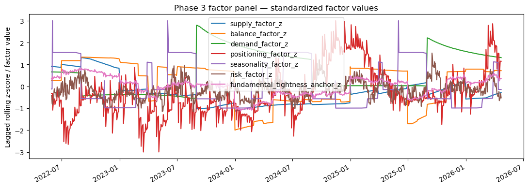
Standardized factor values. The factor panel must be active and time varying.

The second check is whether the factors are too correlated. Some correlation is natural: yield, production, ending stocks, and stocks to use are all connected through the same balance sheet. The goal is not zero correlation. The goal is stable estimation.

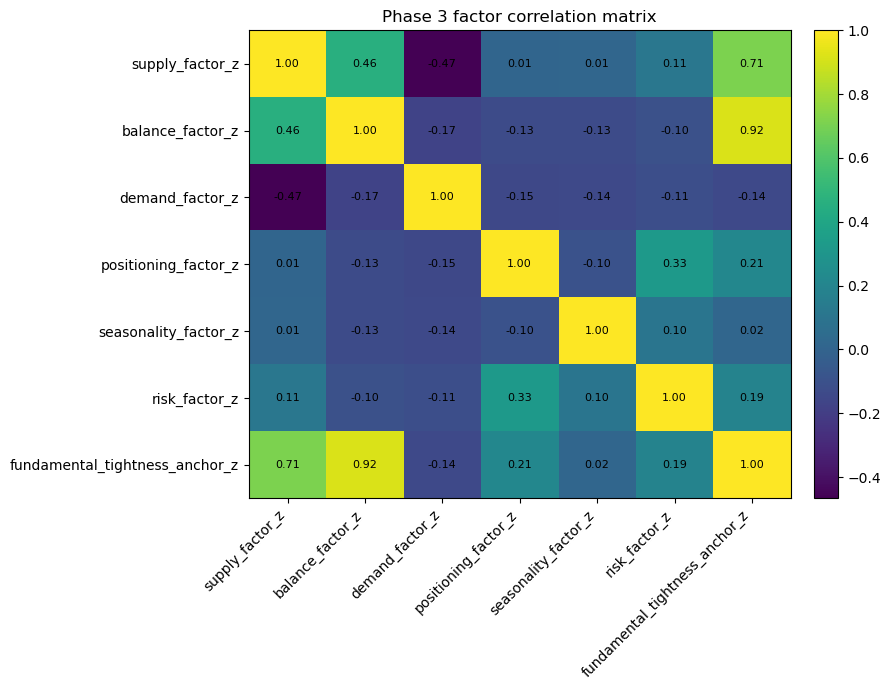
Factor correlations. Economically related factors can be correlated, which motivates ridge regression.

Contract level pricing

A single corn price is not enough. The futures chain contains multiple contracts, $k = 1,2,\ldots,K$.

Each contract has its own expiry, delivery month, curve depth, and exposure to old crop or new crop fundamentals. The model therefore prices contract $k$ at date $t$.

The observed market price is $F_{t,k}$.

The model works in log price because proportional deviations are more stable than raw price deviations, and because storage economics becomes additive in logs. The pricing target is

\[y_{t,k} = \ln(F_{t,k}).\]

The pricing feature vector

The model must explain the log price of a specific contract. A contract price depends on the fundamental factor state, the raw physical state, the contract’s location on the curve, and interactions between the state and the contract.

The feature vector is therefore built from four blocks:

\[X_{t,k} = [\text{Factor State}, \text{Physical State}, \text{Curve State}, \text{Interactions}].\]

The factor state answers how unusual the current corn market state is relative to history. The physical state captures the actual level of the balance sheet. The curve state identifies which contract is being priced. The interactions allow the same economic factor to affect different contracts differently.

The full vector is

\[X_{t,k} = \begin{bmatrix} \text{SupplyFactor}_t \\ \text{BalanceFactor}_t \\ \text{DemandFactor}_t \\ \text{PositioningFactor}_t \\ \text{SeasonalityFactor}_t \\ \text{RiskFactor}_t \\ \text{FundamentalAnchor}_t \\ \text{StocksToUse}_t \\ \Delta\text{StocksToUse}_t \\ \text{ProductionDelta}_t \\ \sqrt{\text{DTE}_{t,k}} \\ \text{DTE}_{t,k} \\ \text{Depth}_{t,k} \\ \text{MonthSin}_k \\ \text{MonthCos}_k \\ \text{SupplyFactor}_t \times \text{DTE}_{t,k} \\ \text{BalanceFactor}_t \times \text{DTE}_{t,k} \\ \text{DemandFactor}_t \times \text{DTE}_{t,k} \\ \text{SeasonalityFactor}_t \times \text{DTE}_{t,k} \\ \text{BalanceFactor}_t \times \text{MonthSin}_k \\ \text{BalanceFactor}_t \times \text{MonthCos}_k \\ \text{SeasonalityFactor}_t \times \text{MonthSin}_k \\ \text{SeasonalityFactor}_t \times \text{MonthCos}_k \end{bmatrix}.\]

Delivery month encoding

Delivery months are cyclical in the same way that crop year days are cyclical. A raw month number treats January as $1$ and December as $12$, which incorrectly makes December and January look far apart even though they are adjacent in calendar time.

Let the delivery month of contract $k$ be $m_k \in {1,2,\ldots,12}$.

Convert the month into a fraction of the annual cycle:

\[v_k = \frac{m_k}{12}.\]

Then convert that fraction into an angle on a full circle:

\[\phi_k = 2\pi v_k.\]

Substituting the month fraction gives

\[\phi_k = 2\pi\frac{m_k}{12}.\]

The sine coordinate of the delivery month is

\[\text{MonthSin}_k = \sin(\phi_k),\]

or

\[\text{MonthSin}_k = \sin\left(2\pi\frac{m_k}{12}\right).\]

The cosine coordinate is

\[\text{MonthCos}_k = \cos(\phi_k),\]

or

\[\text{MonthCos}_k = \cos\left(2\pi\frac{m_k}{12}\right).\]

The expression inside the sine and cosine is the angular location of the delivery month on the yearly contract month circle.

Why interactions are necessary

The same factor should not be forced to have the same price impact on every contract. A supply shock can affect a new crop December contract differently from an old crop July contract. Balance tightness can matter more for nearby contracts when old crop inventory is scarce. Seasonality can matter differently depending on delivery month and days to expiry.

Interaction terms let the model estimate contract specific sensitivities. Start with a direct supply effect. If supply tightness increases, log price may change by a coefficient $\beta_S$:

\[\beta_S\text{SupplyFactor}_t.\]

To allow the supply effect to depend on maturity, add a term that multiplies supply by days to expiry:

\[\theta_S\left(\text{SupplyFactor}_t \times \text{DTE}_{t,k}\right).\]

The supply related part of the model is

\[\beta_S\text{SupplyFactor}_t + \theta_S\left(\text{SupplyFactor}_t \times \text{DTE}_{t,k}\right).\]

Collecting the common factor gives

\[\left(\beta_S + \theta_S\text{DTE}_{t,k}\right)\text{SupplyFactor}_t.\]

The effective sensitivity of contract $k$ to supply tightness is therefore

\[\frac{\partial \ln(F_{t,k})}{\partial \text{SupplyFactor}_t} = \beta_S + \theta_S\text{DTE}_{t,k}.\]

Maturity changes the supply beta.

The same logic applies to delivery month sensitivity. Start with a direct balance effect:

\[\beta_B\text{BalanceFactor}_t.\]

Then allow the balance effect to vary smoothly by delivery month using both cyclical month coordinates:

\[\theta_{B,\sin}\left(\text{BalanceFactor}_t \times \text{MonthSin}_k\right) + \theta_{B,\cos}\left(\text{BalanceFactor}_t \times \text{MonthCos}_k\right).\]

The balance related part of the model is

\[\beta_B\text{BalanceFactor}_t + \theta_{B,\sin}\left(\text{BalanceFactor}_t \times \text{MonthSin}_k\right) + \theta_{B,\cos}\left(\text{BalanceFactor}_t \times \text{MonthCos}_k\right).\]

Collecting the common balance factor gives

\[\left(\beta_B + \theta_{B,\sin}\text{MonthSin}_k + \theta_{B,\cos}\text{MonthCos}_k\right)\text{BalanceFactor}_t.\]

The effective balance sensitivity is therefore

\[\frac{\partial \ln(F_{t,k})}{\partial \text{BalanceFactor}_t} = \beta_B + \theta_{B,\sin}\text{MonthSin}_k + \theta_{B,\cos}\text{MonthCos}_k.\]

The model can now learn that the same balance sheet tightness has different effects across delivery months.

The fitted pricing model

The model maps the contract level feature vector into log price. The simplest linear structure starts with an intercept, adds the weighted feature vector, and leaves an unexplained residual.

For contract $k$ on date $t$, the log price target is $y_{t,k}$, the feature vector is $X_{t,k}$, the coefficient vector is $\beta_t$, and the residual is $\varepsilon_{t,k}$.

The fitted pricing equation is

\[y_{t,k} = \alpha_t + X_{t,k}^{\top}\beta_t + \varepsilon_{t,k}.\]

Since the target is the log futures price,

\[\ln(F_{t,k}) = \alpha_t + X_{t,k}^{\top}\beta_t + \varepsilon_{t,k}.\]

The pricing residual is the part of the market price not explained by fundamentals, physical state, curve state, and interactions.

Why ridge regression is used

The feature set is economically meaningful, but the variables are not independent. Yield affects production. Production affects ending stocks. Ending stocks affect stocks to use. Stocks to use affects the balance factor. Ordinary least squares can therefore become unstable because related variables move together.

The ordinary least squares objective chooses coefficients that minimize historical squared pricing errors. For observation $i$, the model prediction is $\hat{y}_i = X_i^{\top}\beta$.

The pricing error is actual log price minus fitted log price:

\[e_i = y_i - \hat{y}_i.\]

Substituting the fitted value gives

\[e_i = y_i - X_i^{\top}\beta.\]

A positive and a negative error should not cancel each other out, so the error is squared:

\[e_i^2 = \left(y_i - X_i^{\top}\beta\right)^2.\]

At date $t$, the training set contains only observations before date $t$.

The total historical squared pricing error is therefore

\[\sum_{i<t}\left(y_i - X_i^{\top}\beta\right)^2.\]

Ordinary least squares chooses the coefficient vector that minimizes this total squared error:

\[\hat{\beta}^{\text{OLS}}_t = \arg\min_{\beta}\sum_{i<t}\left(y_i - X_i^{\top}\beta\right)^2.\]

The problem is that correlated features can make ordinary least squares coefficients unstable. The model may fit historical prices by using large offsetting coefficients even when those coefficients are not economically reliable.

Ridge regression addresses this by adding a cost for large coefficients. For $p$ features, total coefficient size is measured by the sum of squared coefficients:

\[\sum_{j=1}^{p}\beta_j^2.\]

The strength of the penalty is controlled by the shrinkage parameter $\lambda$.

The ridge penalty is

\[\lambda\sum_{j=1}^{p}\beta_j^2.\]

The ridge objective combines historical pricing error and coefficient shrinkage:

\[\hat{\beta}_t = \arg\min_{\beta}\left[\sum_{i<t}\left(y_i - X_i^{\top}\beta\right)^2 + \lambda\sum_{j=1}^{p}\beta_j^2\right].\]

The first term rewards fit. The second term rewards coefficient stability. A larger $\lambda$ creates stronger shrinkage, while a smaller $\lambda$ makes the model closer to ordinary least squares.

The goal is not only to fit historical prices. The goal is to estimate stable contract level relationships that can be used out of sample.

No lookahead training logic

At date $t$, the model must not use date $t$ market price to train the coefficient that prices date $t$.

The training set available at date $t$ contains only earlier observations:

\[\text{TrainingSet}_t = \{(X_i,y_i):i<t\}.\]

The coefficient vector available for the current prediction is therefore the coefficient estimated from past data, $\hat{\beta}_{t-1}$.

The current fair log price for contract $k$ is computed by applying those past estimated coefficients to today’s feature vector:

\[\hat{y}_{t,k} = X_{t,k}^{\top}\hat{\beta}_{t-1}.\]

Only after the trading decision is made can today’s observation be added to the training set:

\[\text{TrainingSet}_{t+1} = \text{TrainingSet}_t \cup \{(X_t,y_t)\}.\]

This prevents the current market price from contaminating the current fair value estimate.

From fitted log price to fair value

The model estimates fair value in log space. The fitted log price for contract $k$ is $\hat{y}_{t,k}$.

The original price scale is recovered by exponentiating the fitted log price:

\[\text{FairValue}_{t,k} = \exp(\hat{y}_{t,k}).\]

The market price can now be compared with the fitted fair value. An expensive contract satisfies

\[F^{\text{market}}_{t,k} > \text{FairValue}_{t,k}.\]

A cheap contract satisfies

\[F^{\text{market}}_{t,k} < \text{FairValue}_{t,k}.\]

Pricing residual

Because the model is estimated in log space, the pricing residual is also measured in log space. The market log price is $\ln(F^{\text{market}}{t,k})$, and the fitted fair log price is $\hat{y}{t,k}$.

The residual is market log price minus fitted fair log price:

\[\text{Residual}_{t,k} = \ln(F^{\text{market}}_{t,k}) - \hat{y}_{t,k}.\]

A positive residual means the contract is expensive relative to the fitted model. A negative residual means the contract is cheap relative to the fitted model.

Pricing z score

A residual is not tradable until it is scaled by uncertainty. A two cent residual may be large in a quiet regime and irrelevant in a volatile regime. The model therefore estimates the historical residual scale using only past residuals.

Let the residual standard deviation available at date $t$ be

\[\hat{\sigma}_{\text{resid},t} = \text{Std}\left(\text{Residual}_i\right), \qquad i<t.\]

The pricing z score is the current residual divided by the past residual scale:

\[\text{PricingZ}_{t,k} = \frac{\text{Residual}_{t,k}}{\hat{\sigma}_{\text{resid},t}}.\]

This z score is the bridge from valuation to trading.

Calendar spread fair value

The same fitted contract fair values can be used to value calendar spreads. For near contract $n$ and far contract $f$, the observed market spread is

\[\text{MarketSpread}_t = F^{\text{market}}_{t,n} - F^{\text{market}}_{t,f}.\]

The model implied fair spread is built from the fitted fair values of the two legs:

\[\text{FairSpread}_t = \text{FairValue}_{t,n} - \text{FairValue}_{t,f}.\]

The spread error is the observed market spread minus the fitted fair spread:

\[\text{SpreadError}_t = \text{MarketSpread}_t - \text{FairSpread}_t.\]

The spread error must be scaled by spread uncertainty. The first implementation approximates spread uncertainty from leg uncertainty and imposes a minimum floor to avoid treating tiny denominators as high confidence signals:

\[\text{SpreadUncertainty}_t = \max\left(\sqrt{(0.5F^{\text{fair}}_{t,n}\sigma_n)^2 + (0.5F^{\text{fair}}_{t,f}\sigma_f)^2},4.0\right).\]

The spread z score is

\[\text{SpreadZ}_t = \frac{\text{SpreadError}_t}{\text{SpreadUncertainty}_t}.\]

A future improvement should estimate spread residual volatility directly instead of relying on a leg level approximation.

Outright trading rule

The outright trading rule follows the sign of the pricing z score. If the pricing z score is positive, the market price is above fitted fair value and the contract is expensive relative to the model. A sufficiently positive z score creates a short signal:

\[\text{PricingZ}_{t,k} > 0.90.\]

If the pricing z score is negative, the market price is below fitted fair value and the contract is cheap relative to the model. A sufficiently negative z score creates a long signal:

\[\text{PricingZ}_{t,k} < -0.90.\]

The exit rule is based on normalization. Once the absolute pricing z score falls below the exit threshold, the mispricing is no longer large enough to justify the position:

\[|\text{PricingZ}_{t,k}| < 0.30.\]

Spread trading rule

The spread rule follows the sign of the spread z score. If the spread z score is positive, the market spread is above fitted fair spread. The near contract is expensive relative to the far contract, so the strategy shorts the near leg and buys the far leg:

\[\text{SpreadZ}_t > 0.70.\]

If the spread z score is negative, the market spread is below fitted fair spread. The near contract is cheap relative to the far contract, so the strategy buys the near leg and shorts the far leg:

\[\text{SpreadZ}_t < -0.70.\]

The spread exits when the absolute spread z score falls below the normalization threshold:

\[|\text{SpreadZ}_t| < 0.30.\]

Signal selection

On a given date, the model may find both outright and spread opportunities. Each opportunity is scored by the absolute size of its z score:

\[\text{Score} = |Z|.\]

If an outright signal and a spread signal are both available, the implementation prefers the spread when the spread score is close enough to the outright score:

\[\text{Score}_{\text{spread}} \ge 0.90 \cdot \text{Score}_{\text{outright}}.\]

The spread does not need to have a larger score than the outright. It only needs to be close, because spreads isolate relative curve mispricing and reduce broad directional exposure.

Position sizing and risk control

The first implementation uses simple fixed contract sizing. For an outright trade, the unit is $1\text{ contract}$. For a spread trade, the unit is $1\text{ contract per leg}$.

A more general sizing rule should connect position size to signal strength and uncertainty. Signal strength is measured by the absolute z score, $

Z_t

$, while model uncertainty is represented by residual error scale, volatility, or another risk estimate, $\text{ModelUncertainty}_t$.

The desired position size should rise with signal strength and fall with uncertainty:

\[\text{PositionSize}_t \propto \frac{|Z_t|}{\text{ModelUncertainty}_t}.\]

The current implementation also applies practical safeguards. It avoids stale state files, requires finite core factors, waits for enough training data, avoids contracts too close to expiry, limits contract depth, and uses readiness flags for outright and spread trades.

QuantConnect implementation loop

The implementation connects the research state file to the futures chain. At each date, the algorithm reads the available state, obtains the current futures chain, builds contract level features, estimates fair value, computes mispricing scores, decides whether to trade, and only then updates the training set.

The daily loop is

\[\text{Read State}_t \rightarrow \text{Get Futures Chain}_t \rightarrow \text{Build }X_{t,k} \rightarrow \text{Predict FairValue}_{t,k} \rightarrow \text{Compute }Z_{t,k} \rightarrow \text{Trade} \rightarrow \text{Train After Decision}.\]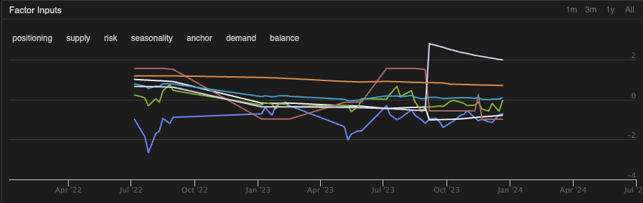

Factor values received by the algorithm: supply, balance, demand, positioning, seasonality, risk, and anchor.

Backtest setup

The first backtest covered the period from $2022$ to $2024$.

The specific start date was January 5, 2022, and the specific end date was April 23, 2024.

Initial capital was $250{,}000\text{ USD}$.

Ending equity was $248{,}352.10\text{ USD}$.

Net profit is ending equity minus starting equity:

\[248{,}352.10 - 250{,}000 = -1{,}647.90\text{ USD}.\]

The percentage return is net profit divided by starting capital:

\[\frac{-1{,}647.90}{250{,}000} = -0.0065916.\]

Converting to percent gives

\[-0.0065916 \times 100 \approx -0.66\%.\]

The backtest summary is:

Metric	Value
Start equity	250,000.00 USD
End equity	248,352.10 USD
Net profit	-1,647.90 USD
Return	-0.66%
Total fees	172.90 USD
Total orders	70
Closed trades	35
Winning trades	22
Losing trades	13
Win rate	62.86%
Loss rate	37.14%
Profit factor	0.8742
Drawdown	1.600%
Sharpe ratio	-3.246
Probabilistic Sharpe ratio	1.606%

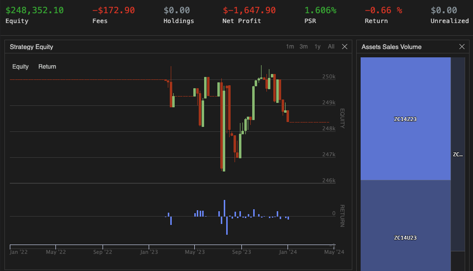
Strategy equity and asset sales volume. The pipeline is active, but the first implementation is not yet profitable.

Backtest interpretation

The backtest produced $35$ closed trades. Of those, $22$ were winners and $13$ were losers. The win rate is winners divided by total closed trades:

\[\text{WinRate} = \frac{22}{35}.\]

Carrying out the division gives

\[\text{WinRate} = 0.6286 = 62.86\%.\]

A win rate above $50\%$ suggests that the signal is not directionally useless. However, profitability depends on both win frequency and payoff size.

The average winning trade was $\text{AverageWin} = 465.91\text{ USD}$.

The average losing trade was $\text{AverageLoss} = -901.92\text{ USD}$.

The payoff ratio compares the average win with the absolute average loss:

\[\text{PayoffRatio} = \frac{465.91}{901.92} \approx 0.5166.\]

The average winner was only about half the size of the average loser.

Expected profit and loss per trade can be approximated from win probability, loss probability, average win, and average loss. The probability of a win is $P(\text{win}) = 0.6286$.

The probability of a loss is

\[P(\text{loss}) = 1 - 0.6286 = 0.3714.\]

The expected trade profit and loss is

\[E[\text{PnL}] = P(\text{win})\cdot\text{AverageWin} + P(\text{loss})\cdot\text{AverageLoss}.\]

Substituting the observed values gives

\[E[\text{PnL}] = 0.6286\cdot465.91 + 0.3714\cdot(-901.92).\]

The winning contribution is approximately

\[0.6286\cdot465.91 \approx 292.80.\]

The losing contribution is approximately

\[0.3714\cdot(-901.92) \approx -335.00.\]

The expected trade is therefore

\[E[\text{PnL}] \approx 292.80 - 335.00 = -42.20\text{ USD}.\]

The main weakness is not the win rate. The main weakness is payoff asymmetry. The current strategy wins more often than it loses, but when it loses, it loses too much.

Current limitations

The first limitation is demand factor quality. Export, ethanol, feed, and total use series require stronger unit checks, timestamp checks, release timing checks, and merge validation.

The second limitation is spread uncertainty. The current implementation approximates spread uncertainty from leg uncertainty. A stronger method would estimate spread residual volatility directly from historical spread errors.

The third limitation is exit logic. The average loss is too large relative to the average win, so exits need to become more volatility aware, more event aware, and more sensitive to residual deterioration.

The fourth limitation is event risk. Major USDA reports can create jumps, so the model should apply special exposure controls around WASDE, Grain Stocks, Prospective Plantings, Acreage, and Crop Production reports.

The fifth limitation is parameter robustness. Entry thresholds, exit thresholds, residual windows, and ridge penalties need systematic testing across regimes.

The sixth limitation is coefficient stability. The fitted betas should be monitored over time to ensure that the model remains economically coherent and is not simply fitting noise.

Main conclusion

The strategy has a coherent economic structure. It begins with the physical corn balance sheet, transforms physical information into signed and standardized economic factors, estimates contract level fair value with a no lookahead ridge model, and trades residual mispricing only when the signal is large enough.

The complete structure is

\[\text{Physical State} \rightarrow \text{Economic Factors} \rightarrow \text{Fitted Contract Fair Value} \rightarrow \text{Mispricing Score} \rightarrow \text{Risk Controlled Trade}.\]

The first implementation is not yet profitable, but it shows that the pipeline works technically. The core empirical result is

\[\text{Win Rate} > 50\%, \qquad |\text{Average Loss}| > \text{Average Win}.\]

The next research priority should therefore be risk side improvement: better exits, volatility aware stops, direct spread uncertainty estimation, event risk controls, and uncertainty adjusted position sizing.