Market Timing as Market Exposure
A decomposition of the Sharpe Ratio of Return Forecasts
A forecast that scores poorly by out-of-sample $R^2$ can still make money. That observation is by now a familiar one, and it carries part of the case for complex return forecasts. What it does not tell you is where the money comes from.
A strategy that scales its position by the forecast earns the average product of the forecast and the return. This cross-moment can be positive even when the forecast is too large or too noisy to reduce squared error. It splits into two pieces: a covariance term, which is timing, and a term equal to the average forecast times the average return, which is exposure to the market premium. Only the first is forecasting ability.
This article runs that split on monthly U.S. data from 1995 to 2025. The market excess return is forecast out of sample with the Welch and Goyal predictors, and the resulting strategy returns are regressed on the Fama and French factors and momentum. In fifteen of eighteen specifications the out-of-sample $R^2$ is negative and the gross Sharpe ratio positive, which is exactly the pattern the complexity literature points to. The covariance term does not differ from zero in any of them. No forecast beats the hit rate implied by sign independence, and once the specification search is counted no deflated Sharpe ratio approaches the conventional threshold. What the strategies earn is exposure to a rising market.
The problem
A known problem in return prediction is the relation between out-of-sample $R^2$, denoted $R^2_{\mathrm{OOS}}$, and expected gross return (Welch and Goyal, 2008; Campbell and Thompson, 2008). The benchmark behind $R^2_{\mathrm{OOS}}$ is the forecast that always predicts zero excess return, that is, the assumption of no predictability. A negative $R^2_{\mathrm{OOS}}$ means the model forecasts worse than this no-predictability benchmark in squared-error terms. In investing, however, this does not always mean the strategy is unprofitable. Kelly, Malamud, and Zhou (2024) rest part of their case for complex forecasts on this point, that a model scoring badly under squared-error loss can still be worth trading. Where that trading return comes from is a separate question.
Out-of-sample $R^2$ measures forecast accuracy. The expected gross return of a strategy depends on how the forecast relates to the future return. Write $\hat{u}_t$ for the forecast and $r_{t+1}$ for the future excess return. A strategy holding a position proportional to $\hat{u}_t$ earns $\hat{u}_t r_{t+1}$, so its expected gross return is governed by the cross-moment $\mathbb{E}[r_{t+1}\hat{u}_t]$ rather than by the forecast error. The strategy can therefore earn a positive gross return when that cross-moment is positive, even if the forecast has negative $R^2_{\mathrm{OOS}}$.
This happens when the forecast points in the right direction but is too large or too noisy to be a good point forecast. It scores poorly under squared-error loss because its own variation is large relative to the signal it carries, yet it can still be economically useful as a trading signal.
A positive gross Sharpe ratio, however, is not by itself evidence of forecasting ability. It is a sample estimate carrying a standard error that widens as the evaluation window shortens, and the largest ratio found across many candidate specifications is inflated by the search itself (Lo, 2002; Mertens, 2002; López de Prado, 2018). A strategy can also earn a positive average return simply because it holds a long position on average in a market with a positive premium, or because it loads on known sources of return such as value, size, momentum, profitability, or investment (Fama and French, 1993, 2015; Carhart, 1997).
Forecast accuracy and trading performance
Let $r_{t+1}$ be the excess return realized over $[t,t+1]$, and let $\hat{u}_t$ be a forecast of it formed at time $t$ and measured in return units. The out-of-sample $R^2$ is
\[R^2_{\mathrm{OOS}} = 1 - \frac{\mathbb{E}\left[(r_{t+1}-\hat{u}_t)^2\right]}{\mathbb{E}\left[r_{t+1}^2\right]},\]the forecast mean squared error relative to the benchmark that always predicts zero. Expanding the square gives the equivalent form
\[R^2_{\mathrm{OOS}} = \frac{2\mathbb{E}\left[r_{t+1}\hat{u}_t\right]-\mathbb{E}\left[\hat{u}_t^2\right]}{\mathbb{E}\left[r_{t+1}^2\right]},\]so accuracy is positive if and only if $\mathbb{E}[\hat{u}_t^2]<2\mathbb{E}[r_{t+1}\hat{u}_t]$. The cross-moment $\mathbb{E}[r_{t+1}\hat{u}_t]$ measures how the forecast relates to the future return, and the second moment $\mathbb{E}[\hat{u}_t^2]$ measures the size of the forecast.
A forecast-scaled strategy uses the forecast as its signal, with weight $w_t=k\hat{u}_t$ for some $k>0$. Its excess return is $r^s_{t+1}=k\hat{u}_t r_{t+1}$, so its expected value is $k\mathbb{E}[r_{t+1}\hat{u}_t]$ and is positive whenever the cross-moment is positive. Profitability thus requires only $\mathbb{E}[r_{t+1}\hat{u}_t]>0$, while accuracy requires the stronger condition above. Between the two lies the region the complexity literature appeals to, where the forecast loses under squared-error loss but still earns money:
\[0<\mathbb{E}\left[r_{t+1}\hat{u}_t\right]<\tfrac{1}{2}\mathbb{E}\left[\hat{u}_t^2\right].\]The forecast may point in the right direction on average, but its magnitude is too large relative to the strength of the signal. The forecast can be economically useful as a trading signal while still being statistically oversized as a point forecast.
The cross-moment separates into two economically distinct sources,
\[\mathbb{E}\left[r_{t+1}\hat{u}_t\right] = \underbrace{\operatorname{Cov}(r_{t+1},\hat{u}_t)}_{\text{timing}} +\underbrace{\mathbb{E}[r_{t+1}]\mathbb{E}[\hat{u}_t]}_{\text{mean exposure}}.\]The first term is genuine timing, the forecast moving with future returns. The second is mean exposure, meaning the strategy earns a positive average return because it has average exposure to a positive risk premium. This decomposition is the one everything below is built on, and it is referred to throughout as the decomposition.
A directionally useful but oversized forecast
Let $r_{t+1}=0.25x_t+\varepsilon_{t+1}$ with $\mathbb{E}[x_t^2]=\mathbb{E}[\varepsilon_{t+1}^2]=1$, and let the forecast be $\hat{u}_t=x_t$. The forecast has the right direction but the wrong scale, since the true coefficient is $0.25$ and not $1$. Its expected gross return for $k=1$ is $\mathbb{E}[r_{t+1}\hat{u}_t]=0.25>0$, so it is profitable. Its out-of-sample $R^2$ is
\[R^2_{\mathrm{OOS}}=\frac{2(0.25)-1}{1+0.25^2}\approx-0.47.\]The same forecast is profitable as a trading signal and poor as a point forecast.
A simulated illustration
The region can be visualized with a simple simulation. Let the future excess return be $r_{t+1}=\beta x_t+\varepsilon_{t+1}$ and the forecast be $\hat{u}_t=a x_t+\eta_t$, where $x_t$, $\varepsilon_{t+1}$, and $\eta_t$ are independent, mean zero, with $\mathbb{E}[x_t^2]=\mathbb{E}[\varepsilon_{t+1}^2]=1$ and $\operatorname{Var}(\eta_t)=\sigma_\eta^2$. Here $a$ is the forecast scale and $\sigma_\eta^2$ is the forecast noise.
The expected gross return for $k=1$ is $\beta a$, which is positive whenever $\beta$ and $a$ share sign. The out-of-sample $R^2$ is more demanding,
\[R^2_{\mathrm{OOS}} = \frac{2\beta a-a^2-\sigma_\eta^2}{1+\beta^2},\]which is positive only when $(a-\beta)^2+\sigma_\eta^2<\beta^2$. With $\beta=0.25$ this holds only for forecasts close to the right scale and with little noise, so most specifications have negative $R^2_{\mathrm{OOS}}$ while still keeping a positive expected gross return. Increasing $\sigma_\eta$ lowers $R^2_{\mathrm{OOS}}$ without changing $\mathbb{E}[r_{t+1}\hat{u}_t]=\beta a$, and increasing $a$ raises the expected gross return linearly while moving $R^2_{\mathrm{OOS}}$ through the concave term $2\beta a-a^2$.
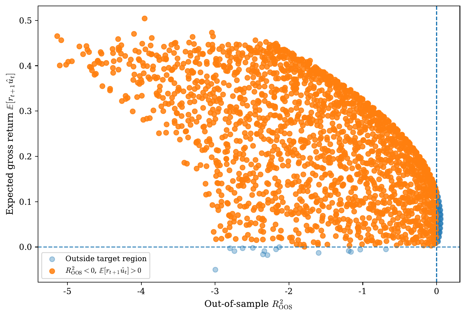 Simulated forecast models, each a pair $(a,\sigma_\eta)$, plotted against out-of-sample $R^2_{\mathrm{OOS}}$ with the expected gross return $\mathbb{E}[r_{t+1}\hat u_t]$ on the vertical axis. Highlighted points have $R^2_{\mathrm{OOS}}<0$ and a positive expected gross return.
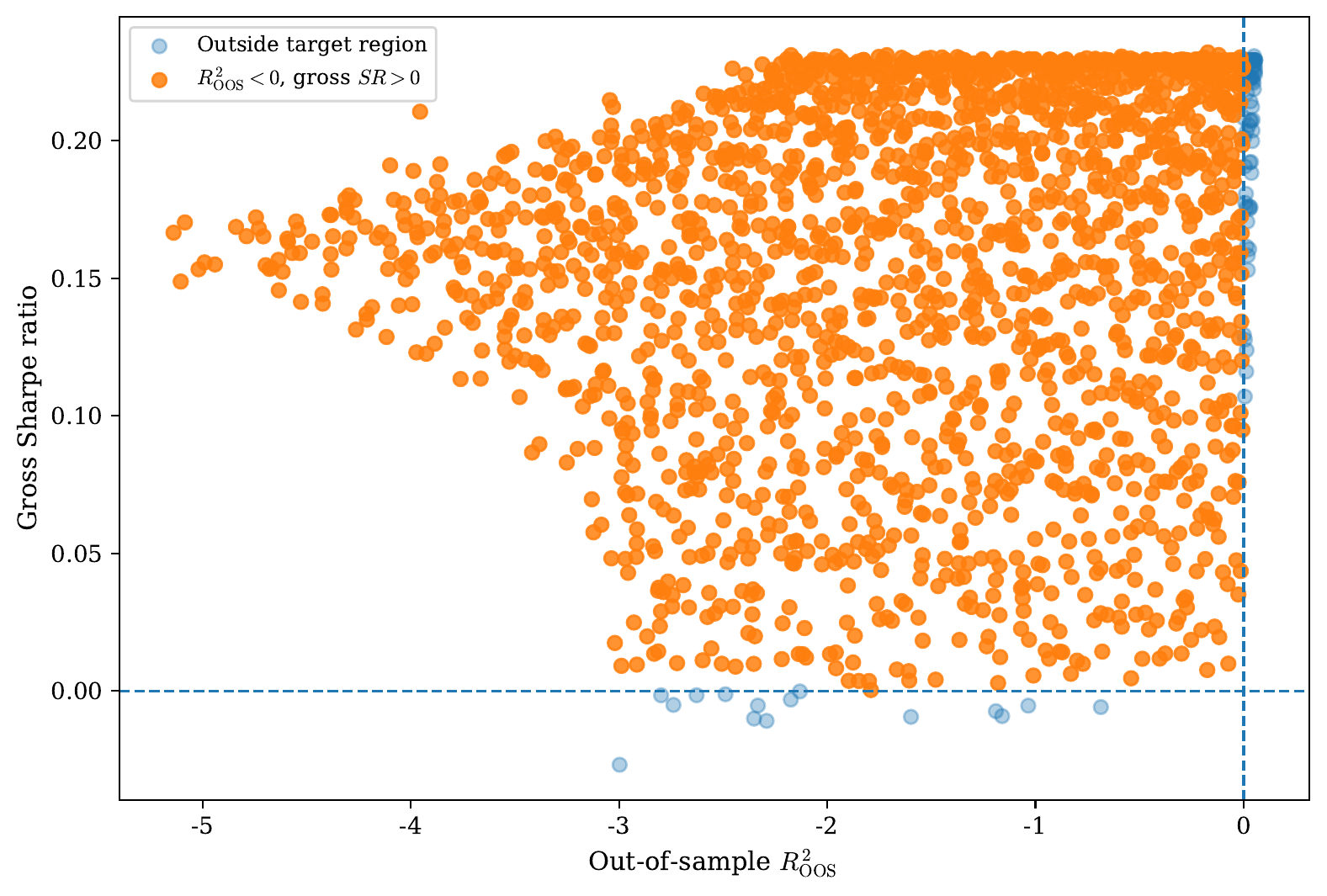 The same models with the per-period gross Sharpe ratio on the vertical axis. With $\beta=0.25$ a positive $R^2_{\mathrm{OOS}}$ needs a forecast near the right scale and with little noise, while any positive scale is enough for a positive cross-moment, so most models fall in the region.
In the Sharpe panel the region fills a wedge with a flat upper edge. That edge is a clean forecast rescaled. With $\sigma_\eta$ near zero, enlarging $a$ is only $x_t$ times a constant, so $R^2_{\mathrm{OOS}}$ slides left while the Sharpe ratio does not move. Noise drops a forecast below the edge, leaving the cross-moment $\beta a$ fixed but inflating the return variance and lowering the Sharpe ratio without ever turning it negative. A forecast reaches a negative $R^2_{\mathrm{OOS}}$ either way, and neither the oversizing nor the noise costs the trade the sign of its signal.
Sharpe ratios and scaling
Since $r_{t+1}$ is an excess return, so is the strategy return $r^s_{t+1}$. Before transaction costs and other frictions, the one-period gross Sharpe ratio is $\mathbb{E}[r^s_{t+1}]/\sigma(r^s_{t+1})$. With $w_t=k\hat{u}_t$ the scaling $k$ cancels, leaving
\[SR_{\mathrm{period}} = \frac{\mathbb{E}[r_{t+1}\hat{u}_t]}{\sigma(r_{t+1}\hat{u}_t)}.\]Its sign is again set by the cross-moment, so a forecast with negative $R^2_{\mathrm{OOS}}$ can carry a positive gross Sharpe ratio.
Scaling makes the contrast precise. Replacing $\hat{u}_t$ by $\alpha\hat{u}_t$ for $\alpha>0$ leaves the Sharpe ratio unchanged, since numerator and denominator scale together. The out-of-sample $R^2$, by contrast, is a concave function of $\alpha$,
\[R^2_{\mathrm{OOS}}(\alpha) = \frac{2\alpha\mathbb{E}[r_{t+1}\hat{u}_t]-\alpha^2\mathbb{E}[\hat{u}_t^2]}{\mathbb{E}[r_{t+1}^2]},\]maximized at $\alpha^{\ast}=\mathbb{E}[r_{t+1}\hat{u}_t]/\mathbb{E}[\hat{u}_t^2]$ and negative once $\alpha>2\alpha^{\ast}$. Accuracy is therefore sensitive to forecast size in a way that trading performance is not.
The sign of the cross-moment, however, does not separate genuine timing from mean exposure. That is what the rest of this article is about.
The empirical decomposition
A positive expected gross return under a negative $R^2_{\mathrm{OOS}}$ is not evidence of timing. By the decomposition, the cross-moment producing it has two sources, and only the first is timing. The two are separated on monthly U.S. data, by forecasting the market excess return out of sample and decomposing the resulting strategy returns against the standard equity factors.
Data
The target $r_{t+1}$ is the monthly market excess return from January 1995 to December 2025, 372 months, taken with the five factors of Fama and French (2015) and momentum (Carhart, 1997) from the French library. The predictors $x_t$ are the fourteen standard variables of Welch and Goyal (2008), taken from the 2025 update of their data set. These forecast the target, while the factors enter only afterwards, to decompose the results.
Forecasts and strategy construction
Every forecast of $r_{t+1}$ is estimated on $\mathcal{T}_t$, the 60 most recent pairs $(x_\tau,r_{\tau+1})$ with $\tau+1\le t$, as are the standardization moments and the ridge penalty. The evaluation runs from February 2000 to December 2025, 311 months.
Let $\sigma_t$ be the standard deviation of the twelve excess returns realized through month $t$, and fit the models to $z_{t+1}=r_{t+1}/\sigma_t$, which holds the variance of the target fixed across the sample. Because this target has constant variance, the forecasts can track only the direction of the return, so any performance they show is direction timing. Each forecast is mapped back as $\hat u_t=\hat z_t\sigma_t$.
The historical mean forecast is the average excess return over $\mathcal{T}_t$,
\[\hat u^{HM}_t = \frac{1}{|\mathcal T_t|}\sum_{\tau \in \mathcal T_t} r_{\tau+1}.\]The combination forecast averages fourteen univariate predictive regressions, one per predictor,
\[\hat u^{C}_t = \frac{1}{14}\sum_{j=1}^{14}\left(\hat a_{j,t}+\hat b_{j,t}x_{j,t}\right),\]as in Rapach, Strauss, and Zhou (2010). The raw multivariate forecast regresses the return on all fourteen predictors at once,
\[\hat u^{OLS}_t = \hat a_t+x_t^{\prime}\hat b_t,\]and the ridge forecast uses the same predictors but shrinks the slope coefficients,
\[(\hat a^{R}_t,\hat b^{R}_t) = \arg\min_{a,b} \sum_{\tau \in \mathcal T_t}\left(r_{\tau+1}-a-x_{\tau}^{\prime}b\right)^2 +\lambda_t\lVert b\rVert_2^2, \qquad \hat u^{R}_t=\hat a^{R}_t+x_t^{\prime}\hat b^{R}_t,\]with the intercept left unpenalized and the penalty $\lambda_t$ chosen by a time-ordered validation split inside $\mathcal{T}_t$. The raw and ridge forecasts differ only through $\lambda_t$, so the comparison isolates the effect of shrinkage.
Each forecast is turned into a forecast-scaled strategy with weight
\[w_t=\frac{\hat u_t}{s_t}, \qquad s_t=\frac{1}{N_t}\sum_{\tau<t}\lvert \hat u_{\tau}\rvert,\]with $N_t$ the number of months before $t$ and $s_t$ the mean absolute forecast over them, so average gross exposure stays near one. It is the $w_t=k\hat u_t$ of the theory, and the strategy return is $r^s_{t+1}=w_t r_{t+1}$. The 60-month window, the 1995 start, and the volatility standardization are choices, and the appendix on specification choices runs the decomposition again under every reasonable alternative.
Accuracy and directional accuracy
Accuracy is measured by the out-of-sample $R^2$ against a benchmark forecast $b_t$,
\[R^2_{\mathrm{OOS}}(b)=1-\frac{\sum_t\left(r_{t+1}-\hat u_t\right)^2}{\sum_t\left(r_{t+1}-b_t\right)^2},\]which reduces to the earlier definition when $b_t=0$. It is reported against the zero benchmark and against the prevailing mean $b_t=\hat u^{HM}_t$, the convention of Campbell and Thompson (2008).
| Forecast | $R^2_{\mathrm{zero}}$ | $R^2_{\mathrm{hist}}$ | Corr | $P(\hat u>0)$ | Hit rate | $P^{\ast}$ | $z$ |
|---|---|---|---|---|---|---|---|
| Historical mean | $-0.020$ | $0.000$ | $-0.042$ | $0.756$ | $0.518$ | $0.565$ | $-2.01$ |
| Combination | $-0.039$ | $-0.019$ | $-0.003$ | $0.852$ | $0.576$ | $0.589$ | $-0.71$ |
| Raw OLS (all 14) | $-3.612$ | $-3.522$ | $-0.139$ | $0.669$ | $0.559$ | $0.543$ | $0.64$ |
| Ridge | $-0.055$ | $-0.034$ | $-0.057$ | $0.797$ | $0.547$ | $0.576$ | $-1.31$ |
Out-of-sample forecast accuracy and directional accuracy, 60-month fixed window, 311 months from February 2000 to December 2025. The zero benchmark forecasts zero excess return, the historical-mean benchmark forecasts the prevailing mean. Corr is the correlation between forecast and realized excess return, and the hit rate is the share of months with matching sign. $P(\hat u>0)$ is the share of months in which the forecast is positive, $P^{\ast}$ the hit rate implied by sign independence, and $z$ the statistic of Pesaran and Timmermann (1992) for the realized hit rate against $P^{\ast}$.
No forecast beats the zero benchmark. The raw multivariate fit is worst at $-3.61$, which is fifteen coefficients fitted on 60 observations, and shrinking it to a ridge raises the $R^2$ to $-0.055$, still below zero.
The hit rates look better than that, and this is where the reading has to be careful. The combination and raw multivariate forecasts hit $0.576$ and $0.559$, with one-sided binomial $p$-values of $0.004$ and $0.021$ against one half. But both forecasts are positive in most months, and the market rose in $0.627$ of them, so a forecast with no timing at all inherits a hit rate near the market’s own up frequency. Every hit rate in the table falls below it. The test of Pesaran and Timmermann (1992) measures each hit rate against the $P^{\ast}$ that sign independence implies, and not one of the eighteen forecasts clears it. The historical mean falls below its own at $z=-2.01$, and the best single predictor reaches no further than $z=0.89$. Even at its optimal scale the ridge forecast reaches an out-of-sample $R^2$ of only about $0.001$, so the forecast carries almost no information about the return, and what looks like performance is mean exposure.
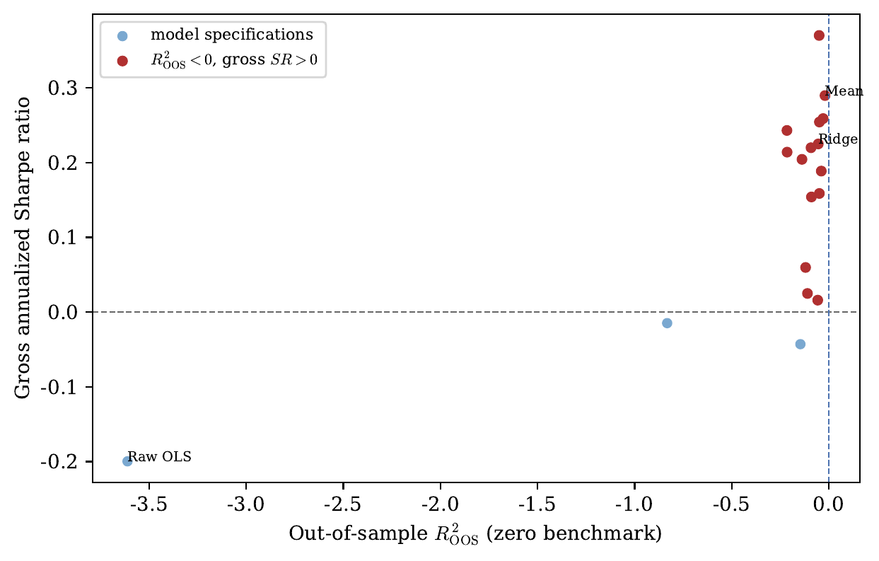 Out-of-sample $R^2_{\mathrm{OOS}}$ against the zero benchmark and gross annualized Sharpe ratio, one point per forecast specification. The highlighted points have $R^2_{\mathrm{OOS}}<0$ and a positive Sharpe ratio. Fifteen of the eighteen specifications fall there: the historical mean, the combination, the ridge forecast and twelve of the fourteen single-predictor forecasts.
Factor decomposition
Each strategy return is regressed on the nested factor sets,
\[r^s_{t+1}=\alpha_q+\beta_q^{\prime}f^{(q)}_{t+1}+\varepsilon^{(q)}_{t+1}, \qquad q\in\{1,3,5,6\},\]where $f^{(1)}$ is the market excess return alone, $f^{(3)}$ is the three-factor set, $f^{(5)}$ is the five-factor set, and $f^{(6)}$ adds momentum. The intercept $\alpha_q$ is the factor-adjusted alpha and the slopes $\beta_q$ are the factor loadings, estimated with Newey and West HAC standard errors. Taking expectations gives
\[\mathbb{E}[r^s_{t+1}]=\alpha_q+\beta_q^{\prime}\mathbb{E}\left[f^{(q)}_{t+1}\right],\]a decomposition of the same kind as before, with $\alpha_q$ the part the factors do not explain and $\beta_q^{\prime}\mathbb{E}[f^{(q)}]$ the part exposure to them earns. Dividing by $\sigma(r^s_{t+1})$ carries the split to the Sharpe ratio,
\[SR=\frac{\mathbb{E}[r^s_{t+1}]}{\sigma(r^s_{t+1})} =\frac{\alpha_q+\beta_q^{\prime}\mathbb{E}[f^{(q)}_{t+1}]}{\sigma(r^s_{t+1})},\]so a positive Sharpe ratio is consistent with a positive $\alpha_q$, and equally with a zero $\alpha_q$ and a positive loading.
For these forecasts it is the second. The three that earn small positive Sharpe ratios show the same source in both decompositions: the covariance term is negative and the factor-adjusted alpha is indistinguishable from zero, so what they collect is the equity premium on an average long position. The raw multivariate strategy is overfit to the point of collapse and sits outside the region entirely.
Kelly, Malamud, and Zhou (2024) regress their timing strategies on the untimed market and report information ratios near $0.3$. The same regression on these four forecasts leaves every alpha indistinguishable from zero, as the market column below shows.
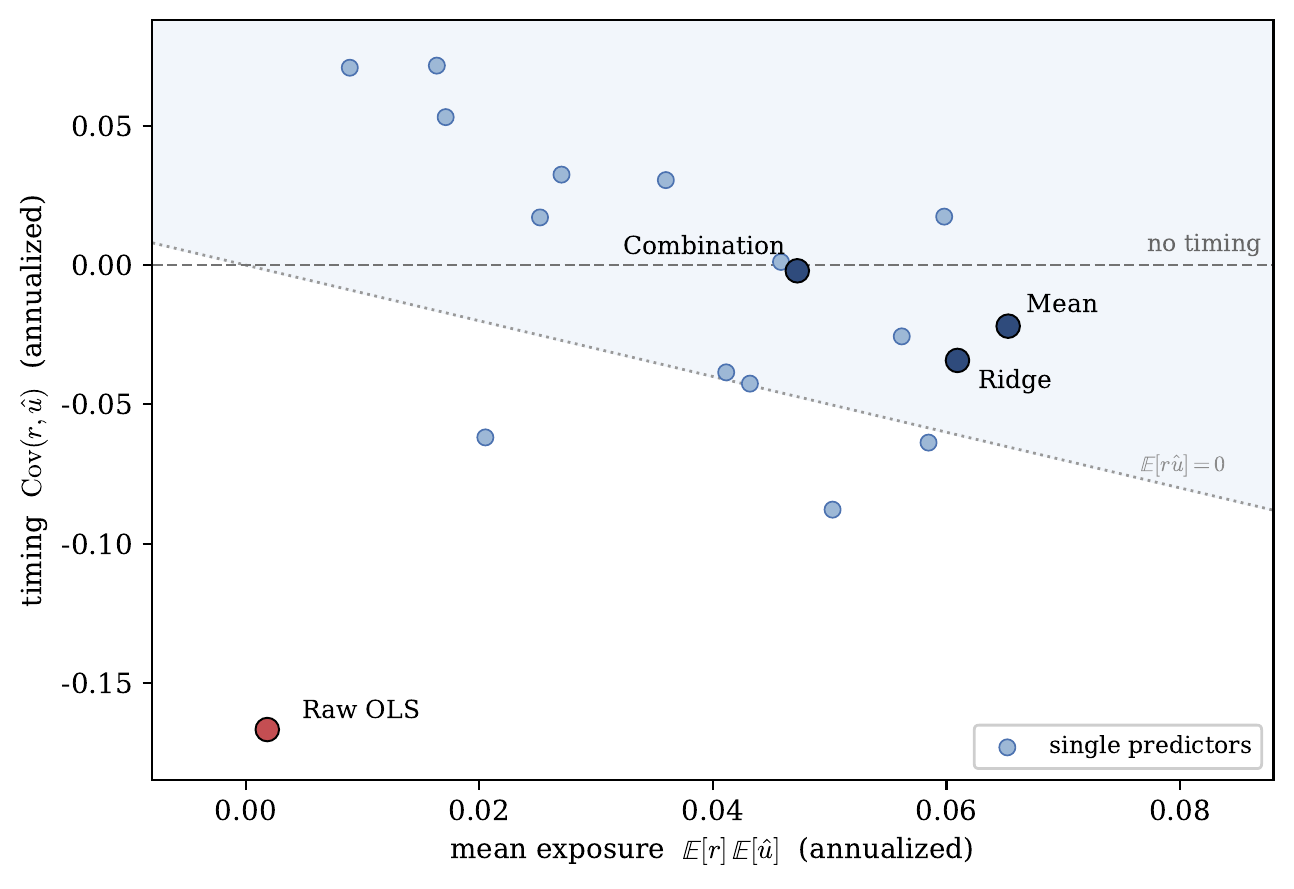 The decomposition for each forecast, at a constant scale. The horizontal axis is the mean-exposure term $\mathbb{E}[r]\mathbb{E}[\hat u]$, the vertical axis the timing term $\operatorname{Cov}(r,\hat u)$, and their sum is the strategy’s mean return. Every forecast has positive mean exposure and timing near zero. The single predictors scatter in timing around zero, of both signs, while the ridge and combination that pool them sit on the no-timing line. The raw multivariate forecast is the exception, near-zero mean exposure with large negative timing. Points above the dotted line $\mathbb{E}[r\hat u]=0$ are profitable.
Every forecast sits at positive mean exposure. The single predictors’ timing scatters both ways and averages out, and the ridge and combination that pool them keep only mean exposure. The raw multivariate forecast is the only one whose timing is large, and it is negative. Tested against zero under Newey and West errors the covariance term carries $t$ statistics between $-1.15$ and $-0.03$, so it is a precise zero.
The absence of timing holds inside market states as well. Splitting the sample at the median of realized volatility and by expansion and recession, the correlation between the ridge forecast and the next return stays negative in all four states, between $-0.03$ and $-0.18$, and the only one that separates from zero is the low volatility half at $t=-2.21$. There is no state in which the forecast times the market.
Taking only the sign of the ridge forecast leaves a Sharpe ratio of $0.04$, so the direction that could time the market adds almost nothing to the position.
| Strategy | Sharpe | Max DD | Market $\alpha$ ($t$) | FF3 $\alpha$ ($t$) | FF5 $\alpha$ ($t$) | FF5+MOM $\alpha$ ($t$) |
|---|---|---|---|---|---|---|
| Historical mean | $0.29$ | $-0.78$ | $-0.23$ ($-0.07$) | $0.07$ ($0.02$) | $-3.69$ ($-1.33$) | $-4.07$ ($-1.40$) |
| Combination | $0.19$ | $-0.91$ | $7.41$ ($0.71$) | $9.30$ ($0.84$) | $4.58$ ($0.55$) | $3.15$ ($0.36$) |
| Raw OLS | $-0.20$ | $-1.00$ | $-11.16$ ($-1.04$) | $-9.15$ ($-0.79$) | $-1.62$ ($-0.19$) | $-5.65$ ($-0.65$) |
| Ridge | $0.22$ | $-0.78$ | $-0.43$ ($-0.13$) | $0.00$ ($0.00$) | $-1.14$ ($-0.37$) | $-1.75$ ($-0.55$) |
Factor decomposition of the forecast-scaled strategies, 60-month fixed window, scaled to an average gross exposure of one. Each factor column reports the annualized alpha in percent with the Newey-West HAC $t$ statistic in parentheses. The market column regresses the strategy on the market excess return alone. Max DD is the maximum drawdown.
Sizing is not timing
The Sharpe ratios above use the trailing scale $s_t$, which varies over time, so the scale invariance of the theory section is exact only for a constant $k$. At constant $k$ the ridge ratio is $0.13$, the same for every constant, and the $0.22$ in the table comes from $s_t$. The two positions have the same volatility, $0.20$ annualized, and the gap is in the mean return, which $s_t$ raises by 70% by carrying more exposure in the months that paid.
| Strategy | Trailing $s_t$ | Constant $k$ | Sign only |
|---|---|---|---|
| Historical mean | $0.29$ | $0.20$ | $-0.05$ |
| Combination | $0.19$ | $0.13$ | $0.22$ |
| Raw OLS | $-0.20$ | $-0.21$ | $0.02$ |
| Ridge | $0.22$ | $0.13$ | $0.04$ |
Sharpe ratios under three position rules. The trailing scale $s_t$ is the rule used throughout. The constant scale fixes $k$ at the full-sample mean absolute forecast. The sign rule holds $\pm 1$ on the sign of the forecast, discarding its magnitude.
The ratios elsewhere use $s_t$, since it is the position the strategy actually holds. But a position whose size moves this way can beat a static benchmark with no timing in it at all, so an alpha against the market cannot say whether a return comes from timing or from sizing. Holding $k$ constant takes the sizing out, and the covariance term is then timing on its own.
None of the four beats the market itself, and since their Sharpe ratios are gross of transaction costs, netting those out would only widen the gap.
What the exposure looks like over time
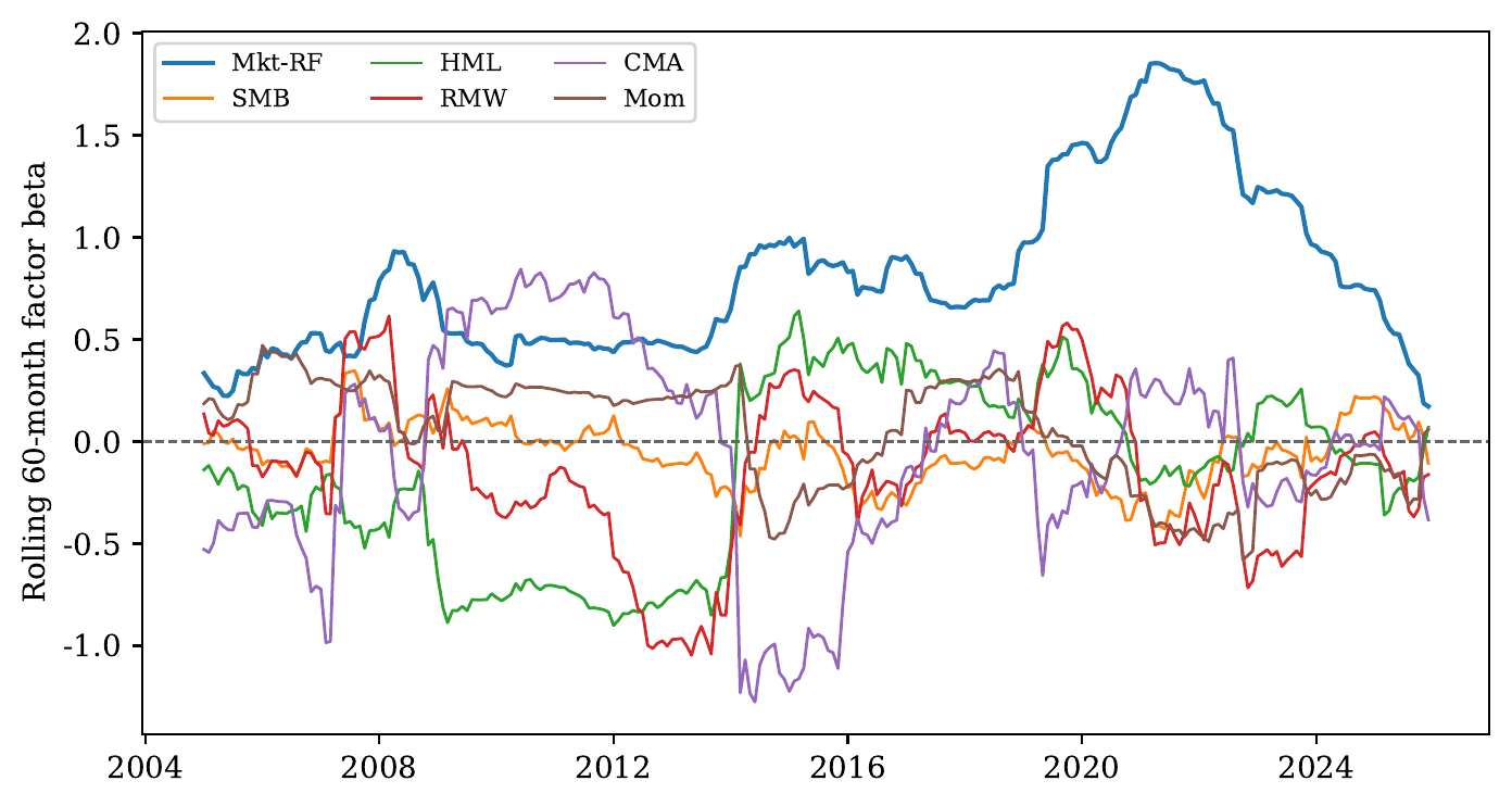 Rolling 60-month factor betas of the ridge strategy against the five factors and momentum. The market beta dominates and averages $0.82$, while the size, value, profitability, investment, and momentum betas all stay near zero. This is the mean exposure term measured over time.
The ridge strategy averages a market beta of $0.82$ through the sample, while its betas on size, value, profitability, investment and momentum all lie between $-0.16$ and $0.04$. The exposure is a long position in the market whose size varies over time.
The market beta rises toward $1.8$ in the window covering the 2020 drawdown and recovery. The scale $s_t$ sets the position from the size of the forecast, and the forecast was large and positive going into 2020, so the strategy ran at close to twice its average exposure and moved with the market at a correlation of $0.86$. That same scale takes no account of market volatility, so the position grew into the 2020 spike and the strategy fell further than the market through February and March before recovering with it. A rolling beta over that window is large only because the average position was large, so the swing traces mean exposure as it moves through time.
The profitability and investment loadings fall toward $-1$ around 2013 and 2014, in windows that still span the 2008 crisis, where the six factors move together closely enough that their individual loadings are not separately identified. The rolling coefficients take large offsetting values while the fitted market exposure holds steady. They swing across $\pm 1$ from one window to the next but average to near-zero levels, so they add nothing to the mean return and only the market term remains.
How much of this survives noise and search
The strategy returns are skewed and fat-tailed, with kurtosis of $11.8$ for the ridge strategy and $87.5$ for the raw multivariate one, so the standard errors below follow Mertens (2002), which corrects the Lo (2002) expression for skewness and kurtosis, estimated under the same Newey and West lag as the factor regressions since the returns carry serial dependence as well. The correction runs in both directions. The positive skewness of the three profitable strategies pulls their errors below the $0.197$ that normal returns would give, and the market’s negative skewness pushes its own above it.
| Strategy | Sharpe | Skew | Kurt | SE | $t$ | 95% interval | PSR | DSR |
|---|---|---|---|---|---|---|---|---|
| Historical mean | $0.29$ | $0.77$ | $9.79$ | $0.19$ | $1.54$ | $[-0.08, 0.66]$ | $0.94$ | $0.55$ |
| Combination | $0.19$ | $2.73$ | $43.10$ | $0.19$ | $1.01$ | $[-0.18, 0.56]$ | $0.84$ | $0.34$ |
| Raw OLS | $-0.20$ | $-7.12$ | $87.52$ | $0.13$ | $-1.58$ | $[-0.45, 0.05]$ | $0.06$ | $0.00$ |
| Ridge | $0.22$ | $1.02$ | $11.78$ | $0.20$ | $1.13$ | $[-0.17, 0.62]$ | $0.87$ | $0.42$ |
| Market (buy and hold) | $0.48$ | $-0.50$ | $3.79$ | $0.22$ | $2.16$ | $[0.05, 0.92]$ | $0.98$ | $0.84$ |
Annualized Sharpe ratios with Mertens standard errors, 60-month fixed window, 311 months from February 2000 to December 2025. The standard error uses the skewness and kurtosis of each strategy return, under a Newey and West kernel at five lags, and would be $0.197$ throughout under normal independent returns. The interval is the 95% confidence interval for the Sharpe ratio. PSR is the probability that the true Sharpe ratio is positive, and DSR the same probability measured against $SR^{\ast}=0.27$ (López de Prado, 2018).
The same errors give the ridge forecast a probabilistic Sharpe ratio of $0.87$, and $0.42$ once the search is deflated. Both fall short of the conventional $0.95$, as do the other three forecasts. The market alone clears it at $0.98$.
The deflation counts the eighteen specifications, whose Sharpe ratios carry a cross-sectional standard deviation of $0.14$, and puts $SR^{\ast}$, the best such a search produces under the null, at $0.27$.
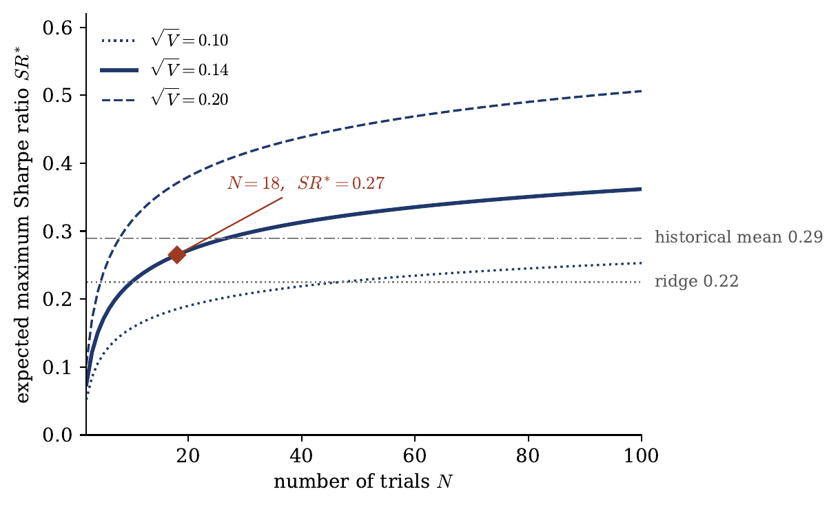 Expected maximum Sharpe ratio against the number of trials, the largest a search of that size reaches when none of its specifications predicts the return. The solid line uses the cross-sectional standard deviation of the eighteen specifications, $0.14$, and the dotted and dashed lines carry it to $0.10$ and $0.20$. The marker is eighteen trials at $SR^{\ast}=0.27$. The horizontal lines are the Sharpe ratios of the historical mean and ridge strategies.
That threshold rises with the number of trials, and the historical mean’s $0.29$ stays above it only until the count reaches 27.
Conclusion
Where the forecasts here make money, none of it is timing. It is the market premium, collected by a position that is long on average. It survives no factor control, and no deflated Sharpe ratio among them reaches the conventional threshold. Over the same period, simply holding the market outright proved more efficient.
This highlights the issue in how such models are evaluated. Trading performance does not validate a forecast unless the return can be attributed to timing. The strategies here offer no return beyond a long position in a rising market. The same decomposition should be applied to any predictive model justified by its economic value. A forecast meant to time the market is better judged by the timing term on its own.
Appendix A: Specification choices and backtest overfitting
Choosing arbitrary parameters would raise concerns about the validity of the results. To settle this, the decomposition is run again under every reasonable window, sample and standardization, and the question is simply whether any of them turns up timing that the baseline missed, once the search across those choices is counted (López de Prado, 2018).
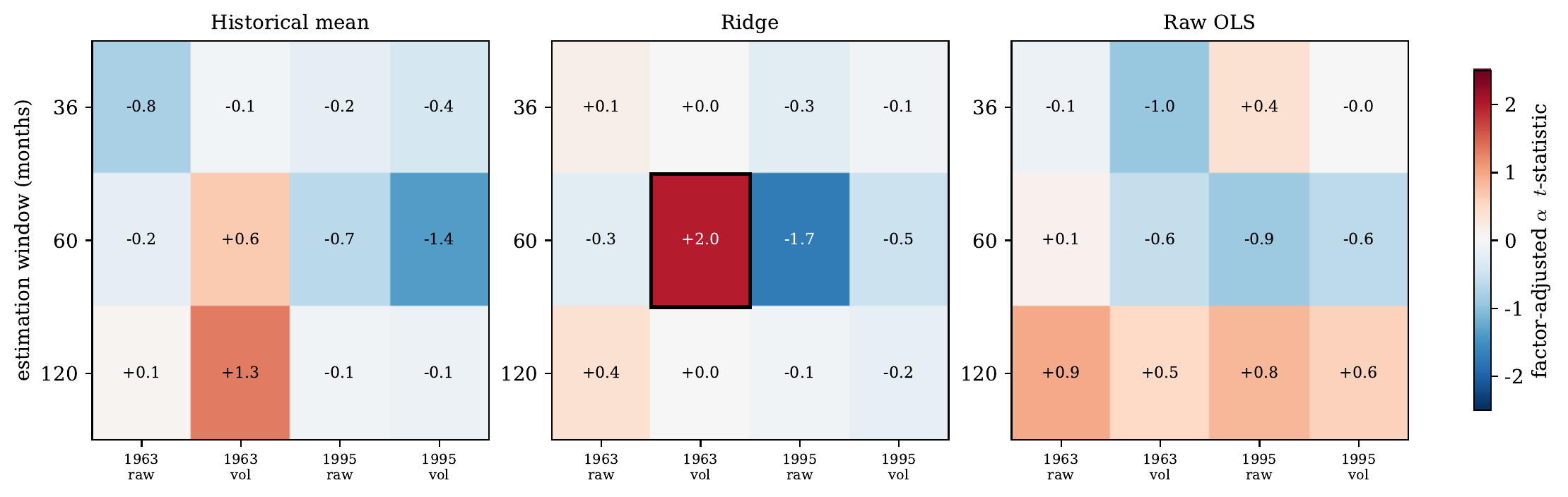 Factor-adjusted alpha $t$ statistic across the estimation window, the sample start and the volatility standardization, for the historical mean, ridge and raw forecasts. Each cell is one out-of-sample run, with the alpha estimated against the five factors and momentum under Newey and West standard errors. Boxed cells exceed $|t|=1.96$. The 1995 columns, the sample used in the article, are insignificant throughout.
| The runs cover windows of 36, 60 and 120 months, samples starting in 1963 and in 1995, and the target in raw or volatility-standardized form. Of the 36 configurations one has $ | t | >1.96$, against the $1.8$ expected under the null of zero alpha throughout. That cell reaches $ | t | =1.97$, in the long sample under volatility standardization, and the probability that 36 independent draws under the same null produce a maximum of $1.97$ or more is $0.83$. |
A combinatorially symmetric cross validation of the factor-neutral returns puts the probability of backtest overfitting at $0.85$, the share of the 924 train and test splits in which the configuration with the highest in-sample Sharpe ratio ranks below the out-of-sample median. Across those splits it averages $0.48$ in sample and $-0.20$ out of it, its out-of-sample ratio is negative in 93% of them, and the regression of the out-of-sample on the in-sample ratio has slope $-0.10$ with $R^2=0.01$.
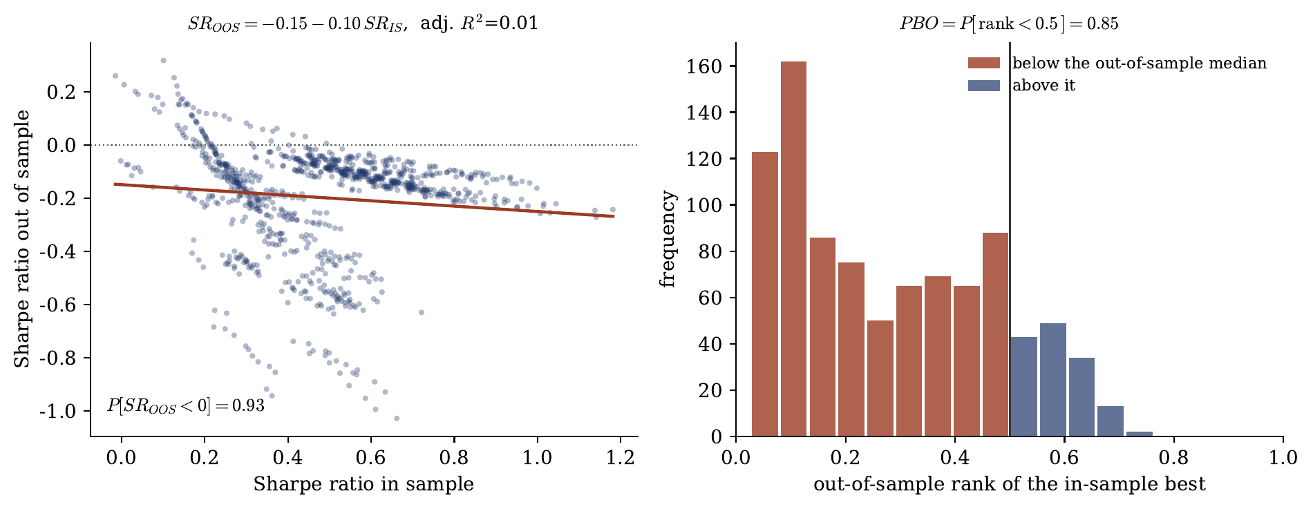 Probability of backtest overfitting by combinatorially symmetric cross validation (López de Prado, 2018), on the factor-neutral returns of the eighteen configurations starting in 1995. The left panel plots the in-sample against the out-of-sample Sharpe ratio of the configuration selected in sample. The right panel is the out-of-sample rank of the configuration chosen in sample, whose mass below the median is the probability of backtest overfitting.
The results do not depend on the parameter choice.
Appendix B: Predictor rank predictivity
The linear forecasts take the predictors as given, so it is fair to ask whether standardizing or squashing them would uncover a signal the regressions leave out. Because rank correlation is invariant to any monotone transform, it already captures whatever a nonlinear adjustment of a predictor could add.
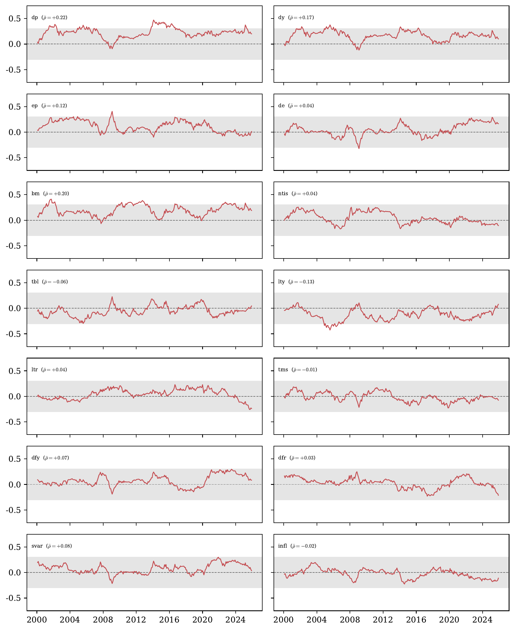 Rolling 60-month Spearman correlation between each Welch and Goyal predictor at $t$ and the next month excess return $r_{t+1}$, February 2000 to December 2025. The shaded band marks $|\rho|<0.3$. The average correlation is $0.06$ and most series sit inside the band throughout.
The rolling correlation averages just $0.06$, and most predictors wander around zero, rarely breaking $\pm 0.3$. The few exceptions are an artifact of persistence. The dividend price ratio, dividend yield, and book-to-market ratio maintain a rolling correlation near $0.2$, but they are statistically indistinguishable from a unit root.
| Predictor | AR(1) $\phi$ | Half-life (months) | ADF $p$ |
|---|---|---|---|
| Dividend price (dp) | $0.977$ | $30$ | $0.24$ |
| Dividend yield (dy) | $0.977$ | $30$ | $0.23$ |
| Book to market (bm) | $0.980$ | $35$ | $0.36$ |
| Earnings price (ep) | $0.974$ | $26$ | $0.00$ |
Persistence of the valuation ratios, sample January 1995 to December 2025. The AR(1) coefficient and the implied half-life of a shock come from a first-order autoregression. The last column is the $p$-value of an augmented Dickey and Fuller test with the null of a unit root.
A shock to these ratios carries an autoregressive half-life near 30 months. Because these series barely move over the evaluation period, a rolling correlation with a drifting market simply traces that same slow drift.
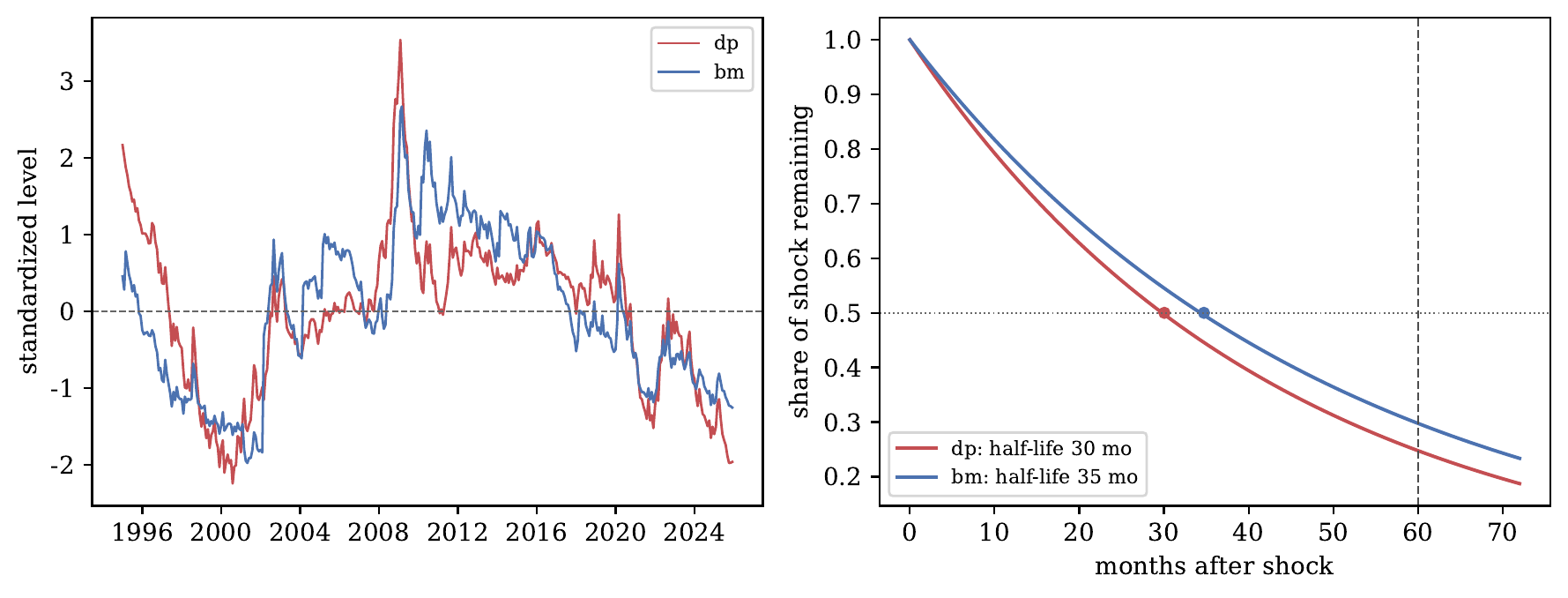 Persistence of the dividend price and book to market ratios. The left plot shows the standardized levels drifting in multi-year swings. The right plot shows the share of a shock that remains over time, with the half-life near 30 months and about a quarter of the shock still present after a full 60-month window, against a typical stationary predictor that is gone within a few months.
Appendix C: Clustered feature importance of the factors
The factor regression is linear, so it is fair to ask whether a nonlinear model would find timing that the regression leaves out. Following López de Prado (2018), a random forest predicts the ridge strategy return from the six factors, and the importance of each is the clustered drop in out-of-sample $R^2$ when it is permuted, on a purged and embargoed $K$-fold. Factors that move together are clustered and permuted as a block, which recovers the importance that a plain per-factor measure would spread across them. It is the same collinearity that leaves the individual loadings unidentified around 2008.
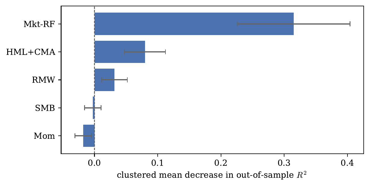 Clustered mean decrease in accuracy for the six factors as predictors of the ridge strategy return, measured out of sample on a purged and embargoed $K$-fold. Importance is the drop in $R^2$ when a factor or cluster is permuted.
The market carries 74% of the importance, and everything else sits at the noise level apart from a value and investment block, HML and CMA, that holds about a fifth. That block is the exposure that swings from window to window in the rolling betas and averages to zero, so it moves the return without adding to its mean. Even with room to fit nonlinearities, the forest finds only market exposure.
References
- Bailey, David H., and Marcos López de Prado. 2014. “The Deflated Sharpe Ratio: Correcting for Selection Bias, Backtest Overfitting, and Non-Normality.” The Journal of Portfolio Management 40(5): 94–107. https://doi.org/10.3905/jpm.2014.40.5.094
- Bailey, David H., Jonathan M. Borwein, Marcos López de Prado, and Qiji Jim Zhu. 2017. “The Probability of Backtest Overfitting.” Journal of Computational Finance 20(4): 39–69. https://doi.org/10.21314/JCF.2016.322
- Campbell, John Y., and Samuel B. Thompson. 2008. “Predicting Excess Stock Returns Out of Sample: Can Anything Beat the Historical Average?” The Review of Financial Studies 21(4): 1509–1531. https://doi.org/10.1093/rfs/hhm055
- Carhart, Mark M. 1997. “On Persistence in Mutual Fund Performance.” The Journal of Finance 52(1): 57–82. https://doi.org/10.1111/j.1540-6261.1997.tb03808.x
- Fama, Eugene F., and Kenneth R. French. 1993. “Common Risk Factors in the Returns on Stocks and Bonds.” Journal of Financial Economics 33(1): 3–56. https://doi.org/10.1016/0304-405X(93)90023-5
- Fama, Eugene F., and Kenneth R. French. 2015. “A Five-Factor Asset Pricing Model.” Journal of Financial Economics 116(1): 1–22. https://doi.org/10.1016/j.jfineco.2014.10.010
- French, Kenneth R. 2026. Kenneth R. French Data Library. https://mba.tuck.dartmouth.edu/pages/faculty/ken.french/data_library.html
- Kelly, Bryan T., Semyon Malamud, and Kangying Zhou. 2022. “The Virtue of Complexity Everywhere.” Swiss Finance Institute Research Paper No. 22-57. https://doi.org/10.2139/ssrn.4171581
- Kelly, Bryan T., Semyon Malamud, and Kangying Zhou. 2024. “The Virtue of Complexity in Return Prediction.” The Journal of Finance 79(1): 459–503. https://doi.org/10.1111/jofi.13298
- Kelly, Bryan T., and Semyon Malamud. 2025. “Understanding the Virtue of Complexity.” Swiss Finance Institute Research Paper No. 25-96. https://doi.org/10.2139/ssrn.5346842
- Lo, Andrew W. 2002. “The Statistics of Sharpe Ratios.” Financial Analysts Journal 58(4): 36–52. https://doi.org/10.2469/faj.v58.n4.2453
- López de Prado, Marcos. 2018. Advances in Financial Machine Learning. John Wiley & Sons.
- Mertens, Elmar. 2002. “Comments on Variance of the IID Estimator in Lo (2002).” Research note, University of Basel.
- Pesaran, M. Hashem, and Allan Timmermann. 1992. “A Simple Nonparametric Test of Predictive Performance.” Journal of Business & Economic Statistics 10(4): 461–465. https://doi.org/10.1080/07350015.1992.10509922
- Rapach, David E., Jack K. Strauss, and Guofu Zhou. 2010. “Out-of-Sample Equity Premium Prediction: Combination Forecasts and Links to the Real Economy.” The Review of Financial Studies 23(2): 821–862. https://doi.org/10.1093/rfs/hhp063
- Welch, Ivo, and Amit Goyal. 2008. “A Comprehensive Look at the Empirical Performance of Equity Premium Prediction.” The Review of Financial Studies 21(4): 1455–1508. https://doi.org/10.1093/rfs/hhm014