Old World vs New World in Expected Returns

I want to reflect on the difference in thinking between the old world and the new world, from risk premia to risk factors to the efficient market hypothesis and rational market participants.

The old world

At the core is the present value relation: an asset’s market price should equal its discounted cash flows. Investors price an asset such that its marginal cost (the price of acquiring it) equals the expected marginal payoff (the expected discounted future payoff).

We can write this as:

\[\begin{equation} P_t = \sum_{T=1}^{\infty} \mathbb{E}_t\!\left[\frac{CF_{t+T}}{(1+r)^T}\right] \label{eq:pv} \end{equation}\]

The cash flows here could be the coupon and principal of bonds or the dividends of equities. The expected cash flow prices in the risk of default and the future path of interest rates. For example, the expected future cash flow of equities reflects the expected future growth rate of dividends or other cash distributions.

But if we look at the denominator of Eq. \eqref{eq:pv}, the discount rate is just another expected return. In equilibrium (i.e., under fair prices), the discount rates investors require are the expected returns they can rationally anticipate. That equilibrium is set by supply and demand among participants using the same equation. The discount rate (equivalently, the expected return) contains both compensation for bearing risk and compensation for time. The riskless rate reflects only the time value of money; Treasury bills are typically used to measure the riskless rate of return in nominal terms.

The expected return of a given asset over the riskless rate is often called the ex ante (risk premium) of that asset.

Assumptions that were later relaxed:

• One period world (this implies a constant investment opportunity set and constant risk premia over time)
• Access to unlimited riskless borrowing and lending, and tradable risky assets
• No taxes or transaction costs
• Rational market participants, i.e., mean variance optimizers (only caring about means and covariances; motivated by normally distributed returns or a quadratic utility function)
• Investors have homogeneous expectations (all agree about the means and variances; i.e., they see the same picture)
• In equilibrium, market clearing requires that the risky asset portfolio demanded in common by all investors equals the market portfolio of risky assets

These assumptions ensure, essentially, that all investors hold some form of the same portfolio of risky assets, combining it with some amount (+/–) of a riskless asset depending on each investor’s risk aversion. Moreover, these assumptions imply that those holdings are optimal in an unrealistic way.

That means, for the CAPM, the asset pricing implication is that assets with higher sensitivity to the market (higher market beta) have higher expected returns. This is a simple rendition of the idea that market participants require compensation for the risk each asset contributes to the portfolio, not for an asset’s standalone risk. Under the assumption that all investors hold the same market portfolio of risky assets, assets with higher market beta contribute more to portfolio risk:

Expected asset return = riskless return + asset beta * market risk premium. More formally:

\[\begin{equation} \mathbb{E}[R_i] = R_f + \beta_i\,\mathbb{E}[R_M - R_f] \label{eq:capm} \end{equation}\]

While these assumptions are false, the idea that only systematic risk is priced (in the sense that it influences expected return) still holds value. Realized returns reflect both systematic risk factors and asset specific (idiosyncratic) risk. The latter is assumed to be diversifiable and thus not rewarded.

The new world

By relaxing the assumptions above, researchers came closer to what the behavior of asset markets actually shows.

In the new thinking of expected return: multiple systematic factors, time varying risk premia, skewness, and liquidity preferences; supply-demand effects, market frictions, and investor irrationalities. No model can capture all effects. Despite diverse new models, all hold one thing in common, one key idea at the core: the asset price still equals expected discounted cash flows. But in a world of uncertainty and time varying expected returns, Eq. \eqref{eq:pv} needs to be generalized.

Price in time (t) for asset (i) is:

\[P_t^i = \mathbb{E}_t\left[SDF_{t+1}\,x_{t+1}^i\right]\]

where (SDF) is the stochastic discount factor and (x) is the payoff (cash flow) for asset (i). The intuition is that the SDF is an index of “bad times”, and the required risk premium for any asset (or risk factor) reflects its covariation with bad times. Investors are willing to pay more, and accept lower expected returns (lower risk premia), for assets that tend to do well in bad times. Conversely, investors require high risk premia for assets that tend to suffer in bad times, and thus pay less for them.

Then the fundamental generalization of Eq. \eqref{eq:capm}, for any risk premium or ex ante excess return, is:

\[\text{Risk premium}_{t}(i) = -\operatorname{Cov}_t\!\left(R_{t+1}^{i,e},\, SDF_{t+1}\right)\]

But how do we define bad times? Formally, bad times are periods when investors’ marginal utility (MU) is high.

Utility

In economics, utility is a measure of a person’s satisfaction from a given state of the world. Over time, the term has been used with at least two meanings.

1. In a normative context, utility refers to a goal or objective that we wish to maximize, i.e., an objective function. This kind of utility bears a closer resemblance to the original utilitarian concept, developed by moral philosophers such as Jeremy Bentham and John Stuart Mill.
2. In a descriptive context, the term refers to an apparent objective function; such a function is revealed by a person’s behavior, and specifically by their preferences over lotteries, which can be any quantified choice.

Consider a set of alternatives among which a person has a preference ordering. A utility function represents that ordering if it is possible to assign a real number to each alternative in such a manner that alternative a is assigned a number greater than alternative b if and only if the individual prefers alternative a to alternative b. In this situation, someone who selects the most preferred alternative must also choose one that maximizes the associated utility function.

Suppose James has utility function (U=\sqrt{xy}), where (x) is the number of apples and (y) is the number of chocolates. Alternative A has (x=9) and (y=16); alternative B has (x=13) and (y=13). Plugging these into the utility function yields:

\[U(A)=\sqrt{9\cdot 16}=12,\qquad U(B)=\sqrt{13\cdot 13}=13,\]

so James prefers alternative B. In general economic terms, a utility function ranks preferences concerning a set of goods and services. For a finite set of alternatives, these require only that the preference ordering is complete (so the individual can determine which of any two alternatives is preferred or that they are indifferent), and that the preference order is transitive.

Suppose the set of alternatives is not finite (for example, even if the number of goods is finite, the quantity chosen can be any real number on an interval). In that case, a continuous utility function exists representing a consumer’s preferences if and only if the consumer’s preferences are complete, transitive, and continuous. Preferences have three main properties:

Completeness

Assume an individual has two choices, A and B. By ranking the two choices, one and only one of the following relationships is true: an individual strictly prefers A (A > B); an individual strictly prefers B (B>A); an individual is indifferent between A and B (A = B). Either a ≥ b OR b ≥ a (OR both) for all (a,b)

Transitivity

Individuals’ preferences are consistent over bundles. If an individual prefers bundle A to bundle B and bundle B to bundle C, then it can be assumed that the individual prefers bundle A to bundle C. (If a ≥ b and b ≥ c, then a ≥ c for all (a,b,c)).

Non satiation or monotonicity

If bundle A contains all the goods that a bundle B contains, but A also includes more of at least one good than B. The individual prefers A over B.[3] If, for example, bundle A = {1 apple,2 oranges}, and bundle B = {1 apple,1 orange}, then A is preferred over B. Economists distinguish between total utility and marginal utility. Total utility is the utility of an alternative, an entire consumption bundle or situation in life. The rate of change of utility from changing the quantity of one good consumed is termed the marginal utility of that good. Marginal utility therefore measures the slope of the utility function with respect to the changes of one good.[9] Marginal utility usually decreases with consumption of the good, the idea of “diminishing marginal utility”. In calculus notation, the marginal utility of good X is M U x = ∂ U ∂ X {\displaystyle MU_{x}={\frac {\partial U}{\partial X}}}. When a good’s marginal utility is positive, additional consumption of it increases utility; if zero, the consumer is satiated and indifferent about consuming more; if negative, the consumer would pay to reduce his consumption. Law of diminishing marginal utility

Rational individuals only consume additional units of goods if it increases the marginal utility. However, the law of diminishing marginal utility means an additional unit consumed brings a lower marginal utility than that carried by the previous unit consumed. For example, drinking one bottle of water makes a thirsty person satisfied; as the consumption of water increases, he may feel begin to feel bad which causes the marginal utility to decrease to zero or even become negative. Furthermore, this is also used to analyze progressive taxes as the greater taxes can result in the loss of utility.

Okay, but this replaces one vague definition with another. What kinds of environments imply high utilities?

It really depends on the asset, model, regime, etc. Here are examples. Consumption based asset pricing models associate bad times with negative consumption growth rates. The intuition of consumption smoothing is powerful: an extra dollar when we are hungry is worth more than when we are satisfied. Recessions are often used as proxies for macroeconomic bad times. Periods of rising and/or high unemployment, rising and/or high inflation, or unexpected monetary policy tightening are other macro states that may be associated with high MU. Financial crises are important high marginal utility (MU) environments, especially if financial institutions have a major role in setting asset prices. If we can equate bad times with stock market losses, we get back the old CAPM; however, “bad times” are likely to be far more multi dimensional. One can attribute other drivers of the crisis, such as vanishing liquidity, bond market selloffs, deleveraging spirals, spiking volatility, and high correlations that suddenly limit diversification benefits, all of which can sharply boost marginal utility even when equity markets appear relatively stable or have not yet fully collapsed. In these episodes, marginal utility rises not only because of falling stock prices (which reduce wealth and consumption opportunities), but because investors and institutions simultaneously face acute constraints on their ability to trade, borrow, or hedge. Liquidity evaporation forces fire sales at depressed prices, deleveraging spirals amplify losses through margin calls and forced unwinding of positions, volatility spikes increase uncertainty and risk aversion, and correlation spikes destroy the diversification that investors rely on in normal times. When financial intermediaries (banks, dealers, hedge funds) are central to price formation, these frictions become self reinforcing: their own balance sheet stress reduces market making capacity, further worsening liquidity and volatility. The result is a state of the world where the effective price of risk is much higher than what a simple equity market downturn would suggest. This multi dimensional nature of crises helps explain why many strategies that appear to have attractive risk premia in normal times (e.g., selling volatility, credit carry, or positive carry trades) can suffer outsized losses precisely when marginal utility is highest.

Empirical test

To bring the idea of multi dimensional “bad times” to the data, I construct a monthly crisis state factor designed to capture financial stress beyond simple equity market declines. The sample runs in practice from 1993 through late 2023, constrained by the availability of the SPY based liquidity proxy and by the differencing used in the PCA step. The objective is to build a single latent factor that rises when several dimensions of market stress worsen together: volatility, funding pressure, credit deterioration, illiquidity, and correlation breakdown. The data come from several sources. Monthly S&P 500 returns and VIX levels are downloaded from Yahoo Finance. The TED spread and the Baa–Aaa corporate bond spread are taken from FRED to proxy for funding and credit stress. To capture trading frictions more directly, I compute an Amihud illiquidity measure using SPY daily data, defined as the monthly average of the daily ratio of absolute return to dollar trading volume. To measure the erosion of diversification benefits during crises, I also construct an average pairwise correlation measure using a representative set of large U.S. equities with long histories (AAPL, MSFT, JPM, JNJ, and XOM), based on rolling daily return correlations.

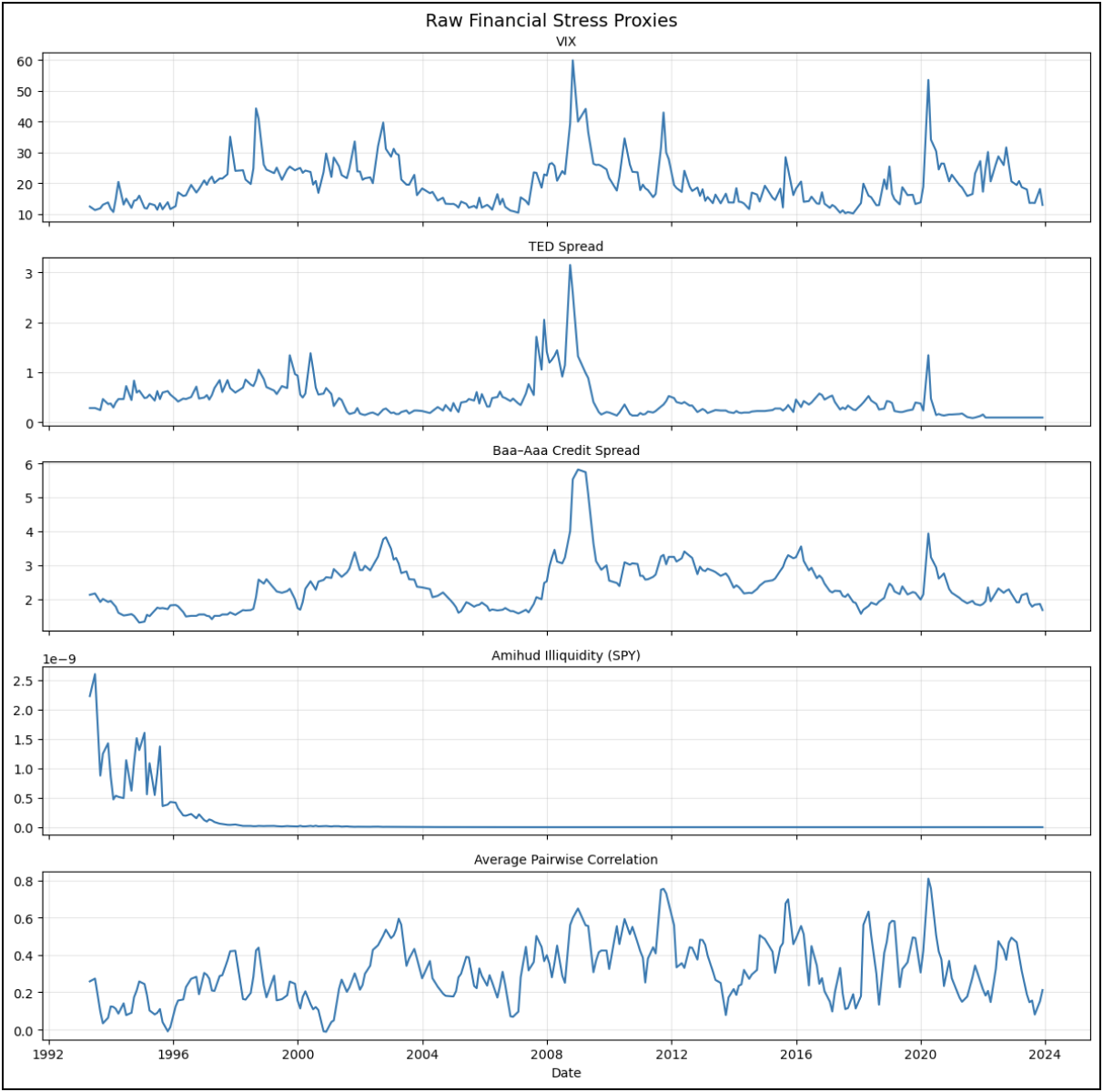Time series of the raw stress proxies

After collecting the raw series, I align them at the monthly frequency and merge them into a common panel. I then focus on monthly changes rather than levels. This is important because crisis conditions are often identified not only by elevated stress, but by sudden worsening in stress. A sharp jump in volatility or credit spreads, for example, is more informative about a transition into a crisis regime than a persistently but quietly high level. The crisis factor is extracted using principal component analysis. Specifically, I take the monthly changes in five variables (VIX, TED spread, Baa–Aaa spread, Amihud illiquidity, and average pairwise stock correlation), standardize them, and estimate the first principal component. This component, denoted (F_{crisis}), is interpreted as the dominant common shock driving multi dimensional financial stress. In the notebook, the first principal component explains about 42.7% of the variance in the standardized changes, which is substantial given that the inputs were chosen to capture related but distinct aspects of stress. The factor loadings are economically sensible. The strongest contributions come from the credit spread and the VIX, followed by pairwise correlation and the TED spread, while the Amihud measure contributes more weakly. This suggests that the estimated factor is driven primarily by worsening volatility and credit conditions, with correlation spikes and funding pressure also playing meaningful roles. In other words, the extracted factor does not simply reproduce stock market losses; it captures a broader regime in which several frictions intensify at once. 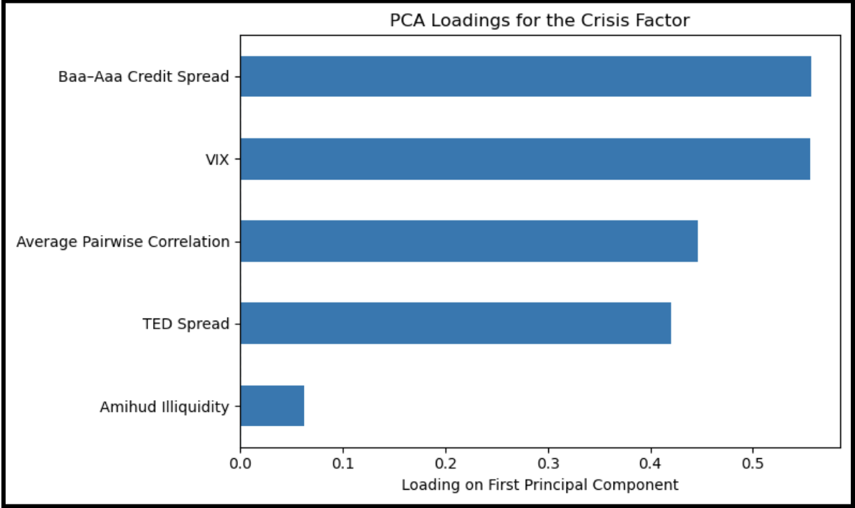PCA loadings for the crisis factor To verify that the first principal component behaves like a crisis variable, I plot its time series and compare it to known episodes of financial strain. The factor spikes sharply around periods such as the global financial crisis and the COVID shock, supporting the interpretation that it captures systemic stress rather than ordinary month to month variation. It also moves with the underlying stress proxies in the expected direction, especially credit spreads and the VIX.

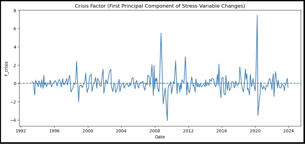Time series of (F_{crisis})

Once the crisis factor is constructed, I test whether it is priced in the cross section of equity returns. For test assets, I use the 25 Fama–French size–value portfolios. These portfolios are useful because they span a broad range of characteristics and have long been used to assess whether proposed factors capture systematic risk missed by the CAPM. For each portfolio, I compute monthly excess returns by subtracting the Fama–French risk free rate. I then estimate the following time series regression:

\(R_{i,t} - R_{f,t} = \alpha_i + \beta_{i,m}(R_{m,t} - R_{f,t}) + \beta_{i,c}F_{crisis,t} + \varepsilon_{i,t}\) where (R_{i,t} - R_{f,t}) is the excess return on portfolio (i), (R_{m,t} - R_{f,t}) is the market excess return, and (F_{crisis,t}) is the latent crisis factor. The regressions are estimated with HAC standard errors using three lags to account for heteroskedasticity and short run autocorrelation in monthly returns. Once standard market exposure is controlled for, do portfolios still differ systematically in how they comove with crisis conditions? If so, and if those crisis exposures line up with average returns, then the CAPM is omitting a relevant priced dimension of risk.

The results indicate that crisis exposure is a distinct and priced source of risk. Across the 25 Fama–French size–value portfolios, crisis betas are widespread and statistically meaningful: 18 of 25 are significant at the 5% level, and 19 of 25 at the 10% level. The most crisis exposed portfolios are Small_Low, Small_High, 2_High, Small_2, and Small_3, while the least exposed are 3_3, Big_3, Big_4, Big_2, and Big_Low. This already suggests that crisis sensitivity is not the same as market beta. The CAPM scatter plot makes this clear. Portfolios with similar market betas often earn different average excess returns, and those differences line up with crisis exposure. Portfolios with higher crisis betas tend to earn higher average returns even when their CAPM market betas are similar, implying that the cross-section is not organized by market risk alone.

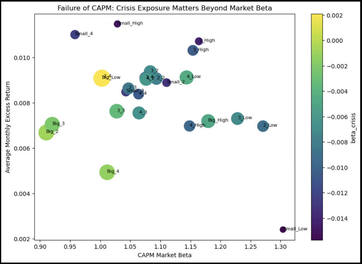CAPM beta vs average excess return, with marker size/color based on crisis beta

Economically, this means investors are compensated not only for comoving with the aggregate market, but also for holding assets that perform poorly when financial conditions deteriorate sharply, when volatility rises, liquidity dries up, credit spreads widen, and correlations spike. These are precisely the states in which marginal utility is highest. The PCA results support this interpretation, since the crisis factor loads most heavily on volatility and credit stress, with additional contributions from funding and correlation measures. It is best understood as a broad financial stress factor rather than a simple equity drawdown measure. The spread portfolio exercise reinforces the same point. After flipping the sign so that higher values of (F_{crisis}) correspond to worse crisis conditions, the natural long–short strategy is to buy portfolios with the highest crisis betas and short those with the lowest. The cumulative return of this high minus low crisis beta spread is consistent with the idea that crisis sensitive assets earn a premium over time for bearing bad times risk.

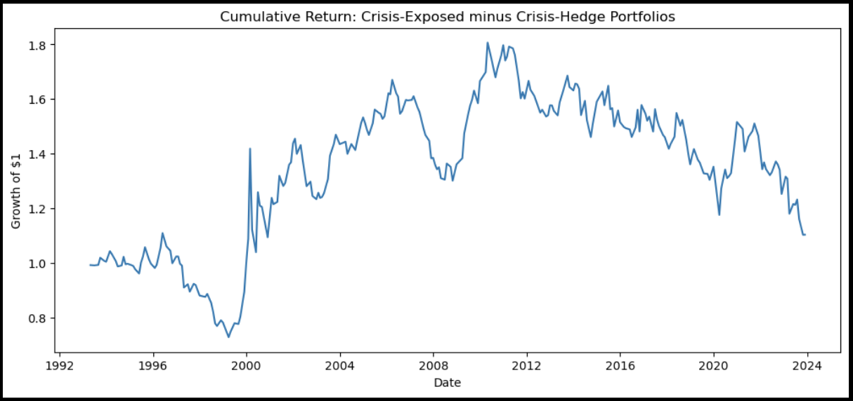Cumulative return of high crisis beta minus low crisis beta portfolios

The evidence suggests that the CAPM is too narrow to capture the full pricing of bad times. A multidimensional crisis factor built from volatility, funding stress, credit conditions, illiquidity, and correlation breakdown helps explain cross-sectional return differences that market beta alone cannot. This supports the broader marginal utility argument: expected returns depend not only on exposure to market movements, but also on exposure to the financial conditions that make crisis periods especially costly for investors and intermediaries.

Table of bad times throughout 1900-now:

Period	Unemployment rate (trough → peak rise)	Equity market (real peak → trough fall)	Description
1929–1932	5% → 22%	–79%	First half of Great Depression
1937–1938	14% → 18%	–49%	Second half of Great Depression
1946–1949	3% → 7%	–39%	Postwar stagnation
1969–1970	3% → 6%	–39%	Stagflationary recession
1973–1975	5% → 9%	–56%	Stagflationary recession
1980–1982	6% → 11%	–28%	Stagflationary recession
2000–2002	4% → 6%	–47%	Dot.com bust, recession
2007–2009	5% → 10%	–52%	Broader bust, recession
1987 Q4	None	–30%	Equity market crash
1998 Q3	None	–18%	Russia/LTCM crisis

Implications for asset pricing and expected returns:

Safe havens like government bonds are not only good diversifiers; they diversify best when it is most needed, hence the name safe havens. In 1998 H2, 2001–2002, 2007 H2–2008, and other episodes, diversifiers fail. Government bonds hedge the equity market best when equities are suffering most, and benefit from flight to quality flows during crises; they may warrant negative ex ante excess return. Although in 2022 government bonds failed spectacularly as safe havens and diversifiers, the episode actually reinforces rather than disproves their value in most crises. That year marked one of the worst periods of positive comovement between stocks and bonds in modern history. U.S. equities (S&P 500) declined about 19% amid slowing growth concerns, while 10-year Treasury yields jumped from roughly 1.5% to over 4.2%. As a result, intermediate and long duration government bonds suffered sharp losses. The Bloomberg U.S. Aggregate Bond Index fell around 13%, and longer Treasuries dropped closer to 17–20%. For the first time in decades, investors experienced simultaneous declines in both major asset classes, erasing the diversification benefit that Treasuries had consistently delivered in prior equity market stress periods such as 1998 H2, 2001–2002, and 2007 H2–2008. The key difference in 2022 was the nature of the shock: persistent, supply driven inflation rather than a classic demand side or financial crisis. Surging inflation (CPI peaking above 9%) triggered aggressive central bank rate hikes to combat price pressures, even as economic growth weakened. Higher policy rates simultaneously raised discount rates for equities and crushed bond prices, flipping the usual negative stock bond correlation into a positive one. In contrast, during typical crises, flight to quality flows drive yields lower and bond prices higher precisely when equities suffer most. This highlights that government bonds provide their strongest hedge exactly when it is needed most, during growth or liquidity driven shocks, but can temporarily lose that insurance value when inflation forces monetary tightening. Even with the rare 2022 exception, bonds often warrant a negative ex ante excess return because of this valuable crisis hedging property. Various strats with asymmetric payoffs (positive carry trades, selling vol and correlation, buying AAA credits vs gov bonds) may be even riskier than their negative skew and fat tails imply. The important point is the timing of losses. Many such strats sell lottery tickets that pay off hugely; they reflect similar fundamental tail risk exposures, but also liquidity induced and positioning induced correlation spikes (especially apparent in 1998, 2008, and 2020).

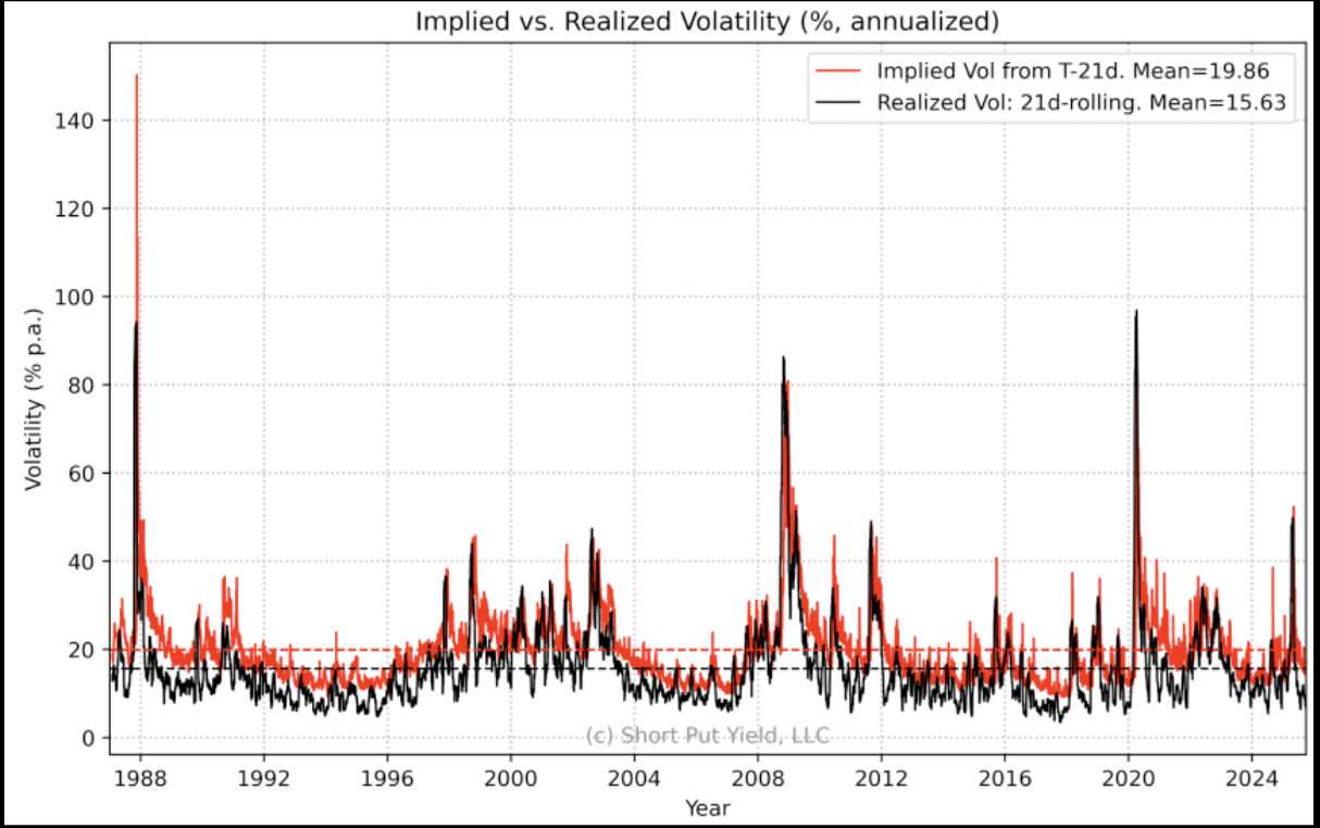the timing of losses in strategies with asymmetric (negative skew) payoffs like positive carry trades, selling volatility, selling correlation, and buying AAA credits vs. government bonds.

We can show empirically that many strats with the best Sharpe since the 1980s are the second type. The covariance with MU is high; they tend to lose in bad times, which could explain their Sharpe.

Important note: many define risk as expected losses and lose the sense of timing. Timing can determine riskiness as much as the amount of losses does, so correlations can matter more than volatility. For example, an investor who started selling volatility right before the crash of 2007–2008 would have been ruined, but someone harvesting gains since 2002 might have survived despite losses, so the MU for the latter is smaller.

Multiple risk factors

We can of course not know the true factor model for “bad times”, so it is tempting to use multi-factor models. Robert Merton’s intertemporal CAPM and Stephen Ross’s arbitrage pricing theory introduced multi-factor models in the 1970s. The Fama–French three-factor model, developed in the early 1990s, has probably replaced CAPM as the most popular model for equity investors.

Recall that according to CAPM, the (i)th asset’s expected return (E_t(r_{t+1}^i)) is a product of its beta, (\beta_t^{iM}), and the market risk premium, (\lambda_t^M), so that:

\(E_t(r_{t+1}^i) = \beta_t^{iM}\,\lambda_t^M\) Beta is the amount of systematic risk in any given asset (thus it varies by asset), and lambda is the market risk premium common to all assets. It can further be deduced that lambda reflects both the amount of risk in the market (stock market volatility) and the price of risk (investors’ risk aversion). It’s restrictive, and doesn’t hold empirically. The tide turned when Fama–French (1992) showed that a “value factor” and a “size factor” (the book to market ratio and market cap as equity characteristics, respectively), rather than factor sensitivities, could explain cross-sectional variation in average equity returns better than a market factor could. The cross-sectional reward for bearing beta risk appears to have been negligible or negative in the CAPM.

To illustrate a multi-factor model, if there are K systematic factors, the ith asset’s expected excess return reflects its respective factor sensitivities (β_i1, …, β_iK) multiplied by the corresponding factor risk premia (λ_1, …, λ_K).

This linear relationship holds under the core assumptions of the Arbitrage Pricing Theory (APT). Asset returns are generated by a K-factor structure, so the theoretical realized excess return of asset i in period t is expressed as:

\[r_{t+1}^i - r_f = \alpha_i + \sum_{j=1}^K \beta_{ij} f_{j,t+1} + \epsilon_{i,t+1}\]

The term f{j,t+1} represents the realized innovation or surprise component of factor *j*, that is, only the unanticipated part of the factor that investors could not have foreseen at time *t*. For example, if the first factor is equity market risk, *f*{1,t+1} is the realized market excess return; if the second factor is inflation risk, f{2,t+1} is actual inflation minus expected inflation. These factor realizations are typically constructed so that their expected value is zero. The residual ε{i,t+1} is the idiosyncratic (asset specific) noise, which by assumption has zero mean, is uncorrelated with the factors, and becomes negligible in well diversified portfolios. Idiosyncratic risk therefore carries no risk premium.

In practice, factors f_{j,t} are identified and constructed in one of three common ways: (1) as directly observed economic surprises (e.g., inflation surprises or industrial production growth), (2) as returns on traded portfolios (e.g., the equity market excess return or the SMB factor), or (3) as statistical factors extracted from a large cross-section of asset returns using principal component analysis (PCA) or similar methods. Once the factors are obtained, betas are estimated asset by asset via the time series regression above, and the risk premia λ_j are recovered from a cross-sectional regression of average asset returns on the estimated betas. This two step (or joint) estimation process turns the theoretical APT pricing equation into an empirically testable model.

Here, the intercept αi is the estimated alpha, the average excess return left unexplained after controlling for all systematic factor exposures. A positive and statistically significant alpha indicates persistent outperformance (abnormal return or pricing anomaly), while a negative alpha signals underperformance. In a correctly specified multi-factor APT model, we expect that in the absence of arbitrage, all expected excess returns are fully explained by the asset’s systematic factor exposures, so α_i = 0 on average. Any non zero alpha would represent a pricing anomaly that investors could exploit to earn riskless profit. Empirically, however, alpha is often not zero. A non zero alpha may reflect true manager skill, a missing risk factor not captured by the model, or statistical noise. The residual ε{i,t} remains the period by period idiosyncratic noise (mean zero by construction), whereas alpha captures any systematic shift or persistent mispricing across the entire sample period.

Additional key assumptions include the existence of well diversified portfolios (a large number of assets relative to the number of factors) and the absence of arbitrage opportunities. In equilibrium, any deviation from the linear pricing relation in a well-diversified portfolio would allow construction of a zero net investment, zero systematic risk portfolio with positive expected return, an opportunity that cannot persist. The factors themselves must be pervasive and systematic, affecting many assets simultaneously so that their risk cannot be eliminated through diversification.

These assumptions are considerably weaker than those of the CAPM, as the multi-factor framework does not require mean-variance optimization, homogeneous investor expectations, or reliance on a single market portfolio. It can hold even when investors have differing beliefs or utility functions, provided arbitrage forces keep prices aligned with the factor exposures.

The expected excess return of any asset (or strategy) is explained by how much exposure (the betas) it has to each rewarded systematic risk factor, scaled by the market’s compensation per unit of that risk (the lambdas). Assets or strategies with higher betas to high λ factors, such as equity market risk, value, carry, volatility selling, or liquidity risk, should therefore deliver higher long run expected returns.

We can take an example of a simple two-factor model with equity market risk and inflation risk. The expected excess return for any asset equals thus, E_t(r_t+1^i) = B_t^i1 * lambda_t^1 + B_t^i2 * lamda_t^2 Where B_t^ij is the asset ith sensitivity to factor j (in this case j=1 is equity market, and j=2 is inflation) and lambda is the factor risk premium (market price of risk)for factor j. So the realized per period excess return can be expressed as a sum of the two systematic exposure plus an uncorrelated residual term

\[r_{t+1}^i - r_f = \beta_{t}^{i1} f_{1,t+1} + \beta_{t}^{i2} f_{2,t+1} + \epsilon_{i,t+1}\]

In practice, we test the model by estimating the following time series regression on historical data (which deliberately includes an intercept to check whether the theoretical no arbitrage condition holds):

\[r_t^i - r_f = \alpha_i + \sum_{j=1}^K \beta_{ij} f_{j,t} + \epsilon_{i,t}\]

Fama–French three-factor model

A prominent empirical implementation of the multi-factor approach is the Fama-French three-factor model, developed by Eugene Fama and Kenneth French in their 1992 and 1993 papers. The model arose directly from the well documented empirical shortcomings of the single factor CAPM. Over many decades, researchers observed that market beta alone explained surprisingly little of the cross-sectional differences in average stock returns. Two persistent patterns stood out: (1) stocks of small capitalization companies tended to deliver higher average returns than large-cap stocks, even after adjusting for market beta (the “size effect”), and (2) “value” stocks, those with high book to market equity ratios, tended to outperform “growth” stocks with low book to market ratios (the “value effect”). These patterns could not be reconciled with the CAPM, which predicted that only market beta should matter. In fact, the reward for bearing market beta risk often appeared weak or even negative once these characteristics were accounted for. Fama and French therefore asked a deeper question: could these two firm characteristics (size and book to market) be proxying for additional systematic risk factors that investors care about, beyond simple market risk? Small stocks and value stocks might be riskier in certain “bad times” that are not fully captured by broad market declines, for instance, periods of financial distress, liquidity stress, or economic slowdowns when marginal utility is particularly high. Investors rationally demand higher expected returns (risk premia) for bearing exposure to these extra dimensions of risk. To capture this idea empirically, Fama and French constructed two new factor mimicking portfolios using a systematic sorting procedure on the universe of U.S. stocks (typically all NYSE, Amex, and NASDAQ stocks):

They first sorted stocks into two size groups using the median NYSE market capitalization as the breakpoint: small (below median) and big (above median). Independently, they sorted stocks into three book to market groups: low (bottom 30%, growth), medium (middle 40%), and high (top 30%, value).

This double sort created six value weighted portfolios (Small/Low, Small/Medium, Small/High, Big/Low, Big/Medium, Big/High). From these six portfolios they built two zero net investment (long-short) factors:

SMB (Small Minus Big): the average return of the three small portfolios minus the average return of the three big portfolios. This isolates the return premium associated with firm size, holding other characteristics roughly constant. HML (High Minus Low): the average return of the two high book to market (value) portfolios minus the average return of the two low book to market (growth) portfolios. This isolates the return premium associated with value characteristics.

Both SMB and HML are constructed monthly and represent the excess return an investor would earn by tilting toward small/value stocks while shorting large/growth stocks. Under the assumption that these factors proxy for pervasive systematic risks (rather than pure mispricing), their average returns (λ_SMB and λ_HML) represent compensation for bearing those risks. Starting from the CAPM baseline, (E(r_i - r_f) = \beta_{iM}\cdot \lambda_M), and adding the two new factors leads naturally to the three-factor pricing equation. The expected excess return of asset (i) is now a linear combination of its sensitivities to all three factors, each multiplied by the respective risk premium: \(E(r_i - r_f) = \beta_{iM} \cdot \lambda_M + \beta_{iSMB} \cdot \lambda_{SMB} + \beta_{iHML} \cdot \lambda_{HML}\) Here:

• (\beta_{iM}) measures the asset’s sensitivity to the market factor (broad equity market excess return).
• (\beta_{iSMB}) measures its sensitivity to the size factor (how much the asset behaves like small-cap stocks).
• (\beta_{iHML}) measures its sensitivity to the value factor (how much it behaves like high book-to-market stocks).
• (\lambda_M), (\lambda_{SMB}), (\lambda_{HML}) are the prices of risk (average excess returns) for the market, size, and value factors, respectively.

An asset with high positive loadings on SMB and HML (i.e., one that comoves strongly with small and value stocks) should offer higher expected returns because it provides less diversification precisely when investors’ marginal utility is elevated, during distress or liquidity driven crises. The model assumes that these three factors are sufficient to span the relevant systematic risks for equities, that idiosyncratic risk (ε) is diversifiable and carries no premium, and that no arbitrage opportunities remain once exposures to all three factors are accounted for. Empirically, Fama and French tested the model using time-series regressions on portfolios double-sorted by size and book to market. They found that the three-factor model explained roughly 90% or more of the variation in average returns across diversified portfolios, a substantial improvement over the CAPM. Most of the alphas (intercepts) that were large and significant under the CAPM became close to zero, indicating that what previously looked like abnormal performance was largely compensation for size and value risk exposures.

Back to the point

Within the Stochastic Discount Factor (SDF) framework, once we have derived the expected excess return of an asset as:

\[\text{Risk premium}_{t}(i) = -\operatorname{Cov}_t\!\left(r_{t+1}^{i,e},\, SDF_{t+1}\right)\]

we can directly price any asset by taking the expectation:

\(P_t^i = \mathbb{E}_t\!\left[SDF_{t+1}\,\text{payoff}_{t+1}^i\right].\) This is the generalized present value relation that replaces the old constant discount rate formula. It allows us to “discount” future payoffs using a random (state dependent) discount factor instead of a fixed rate. If we assume that the SDF itself is linearly related to a set of common risk factors, then asset returns can be shown to follow a linear multi factor model. The SDF framework and the linear factor models (such as APT or Fama-French) are complementary: the SDF provides the economic motivation for why risk is priced, while the linear factor model provides a practical statistical representation for implementation. Moreover, the same logic that applies to individual assets also applies directly to the risk factors themselves. The risk premium of any factor (for example, the equity market factor, the value factor HML, or a volatility selling factor) is equally determined by its own covariance with the SDF. A factor that tends to deliver poor returns precisely when marginal utility is high (i.e., in bad times) will command a large positive risk premium. Conversely, a factor that performs well in bad times (such as a liquidity providing or safe haven factor) will have a low or even negative risk premium. This connection shows that the multi-factor models we use in practice are not arbitrary. They are theoretically grounded in the SDF view of “bad times.” When we estimate betas on SMB, HML, or other factors, we are indirectly measuring how much each factor covaries with marginal utility. Strategies that load positively on factors with high SDF covariance (i.e., factors that crash in crises) will therefore earn high expected returns, but they will also suffer their largest losses exactly when investors value money the most. This explains why many high-Sharpe strategies since the 1980s (such as selling volatility or credit carry) look attractive on average but can be far riskier than their volatility or skewness alone suggests: their losses are concentrated in the highest marginal utility states. So if we view bad times as underlying concept, the sign/size of each factors market price of riskreflects the covariance with this meta concept. Alternatively, we can treat different dimensions of bad times as distinct factors, each factor defines different though overlapping, set of high MU periods that the average investor cares about. So investors who bear these priced factor risks effectively supply insurance to other investors against enduring losses in bad times and earn a factor risk premium as compensation for it.

What factors?

Enough, what factors?? Anything. Intertemporal models provide some direction, since theory doesn’t give that guidance. Merton’s CAPM implies that priced factors other than market beta should hedge against future changes in the investment opportunity set. As investment opportunities vary over time, required returns depend on their covariation with future investment opportunities. Merton suggests the long bond rate as a factor, since all investors are exposed to the risk that they will not be able to invest at current rates. The factors chosen to model with does thus simply not depend on theory, they instead are fit empirically, fama-french value factor could be justified as it reflects pronounced distress riska d size factor may reflect illiquidity. To sum it simply, empirical factors explains statistically better the cross sectional and time series variation in asset returns, while theoretically grounded ones explain why factors that are identified explain their risk premia. Empirical models relate average returns to certain risk-factor sensitivities (covariance) or directly to asset characteristics (value, size, etc.).

In that case how to deduce which risk factors?

So one can identify risk factors by examining which factors, from a given set, are effective at explaining realized return variation over time, and then determine whether these factors are cross-sectionally priced (by looking at averages of assets with high and low exposures to that factor and seeing whether average returns differ). Another way is simply asset characteristics, and even if it seem worse than factor sensitivities, they might fit the job better as they are often less noisy measures of true factor risk exposures than historically estimated factor sensitivities.

Factors in asset pricing models can be grouped into two broad categories: those with solid theoretical foundations rooted in economic mechanisms and those discovered primarily through empirical patterns in historical returns. Theoretically grounded factors arise from structural models that connect asset prices to real economic risks. Examples include investment growth factors in production-based asset pricing models. These models, inspired by q-theory, show that firms’ optimal investment decisions imply lower expected returns for companies that invest aggressively today (high asset growth or capital expenditure), as they effectively face lower marginal costs of capital. Another important set comes from labor-related risks. Since human capital represents the dominant source of wealth for most households, factors linked to aggregate labor income growth and idiosyncratic job risk (or unemployment risk) play a central role. Assets that perform poorly when labor markets deteriorate, when wages stagnate or job losses rise, tend to command higher risk premia because they fail to hedge the non-tradable risk that matters most to investors. In contrast, many widely used factors are largely empirical, identified because they explain cross-sectional differences in average returns better than existing models, even if a clean theoretical story came later (or remains incomplete). The classic examples are the size (SMB) and value (HML) factors from the Fama-French three-factor model, which capture the outperformance of small-cap stocks and high book to market (value) stocks beyond what market beta can explain. Momentum, often added as a fourth factor in the Carhart model, is another prominent case: recent winners continue to outperform recent losers, a pattern driven strongly by return evidence rather than a single unifying theory, though behavioral explanations involving underreaction or investor psychology are common. The search for such patterns has produced an explosion of documented factors, so many, in fact, that John Cochrane famously described the situation in 2011 as a “factor zoo.” Researchers have proposed hundreds of candidates over the decades, raising concerns about data mining, overfitting, and the risk that many are simply statistical artifacts rather than genuine sources of compensated risk. Cross-sectional predictability studies have revealed a long list of additional empirical factors and characteristics, including short-term and long-term return reversals, idiosyncratic volatility, various measures of liquidity (illiquidity premia for harder to trade securities), financial distress or bankruptcy risk, earnings momentum and analyst forecast revisions, quality related signals such as accruals (firms with more aggressive accounting tend to underperform), profitability (robust versus weak operating profitability), conservative versus aggressive investment, and corporate actions like asset growth, net share issuance, and payout policy. Other candidates that frequently appear include betting against beta (low risk anomaly), seasonality effects, and various mispricing or limits to arbitrage proxies. Beyond equities, different asset classes bring their own systematic risk factors. In fixed income, interest rate risk (term or duration exposure) and credit risk (default and spread risk) dominate, while an inflation factor is especially critical for nominal bonds because unexpected inflation erodes real payoffs. International and emerging market securities introduce dollar risk (currency fluctuations), and other classes feature factors such as commodity carry, volatility risk, or mortgage prepayment risk in securitized products. In practice, many investors and researchers combine theoretical and empirical factors inside the stochastic discount factor or multi-factor framework. Ultimately, a factor’s risk premium is determined by how strongly it covaries with marginal utility, in other words, how severely it suffers in high marginal utility “bad times.” Factors tied to labor income shocks, investment distress, liquidity dry-ups, or credit crises therefore tend to offer sizable compensation, but they also expose portfolios to precisely those painful states when investors value an extra dollar the most. The sheer size of the factor zoo underscores both the richness of asset pricing research and the ongoing challenge of distinguishing genuine risk premia from noise.

What matters, in the end, is not whether a factor has a tidy name or a neat backtest, but whether it corresponds to a trade-off that survives outside the sample. That means tracking how and when it pays, how it fails, and how it interacts with constraints that show up precisely when capital is most scarce.